Optimization
Convexity
Derive convex sets from mixing production plans, distinguish convex functions from feasible regions, and connect global minima to quadratic curvature.
Mixing production plans: what remains possible?
Suppose two production plans both respect a factory’s capacity and produce matching parts. Can we spend half the time following each plan and still satisfy those requirements? Convexity of a set says that every such mixture stays in the set. Convexity of a function adds a different requirement: the value at a mixed input is no greater than the corresponding average of endpoint values. See Boyd and Vandenberghe’s set definition, slide 2.3, and function definition, slide 3.1.
We begin with Kantorovich’s published production problem, already solved in Linear programming. This is an application of convexity to a historical optimization problem, not a claim that convexity originated with that example. The calculations and proofs on this page are our modern re-derivations; supplementary invented examples are identified separately.
The published rates and the divisible-time model
Kantorovich’s 1939 monograph asks how to divide machine time to maximize completed items, each consisting of one Part I and one Part II. His Example 1 and Table 1 give these rates; he explicitly calls the data illustrative, rather than observations from an actual factory. See pp. 369–370 of the English translation.
| Group | Available machine-days | Part I per machine-day | Part II per machine-day |
|---|---|---|---|
| Milling | 3 | 10 | 20 |
| Turret lathes | 3 | 20 | 30 |
| Automatic turret lathe | 1 | 30 | 80 |
A machine-day is one machine working for one day. Let $m,t,a$ be the machine-days assigned to Part I in the three groups. The remaining times $3-m,3-t,1-a$ make Part II. Time is divisible, all available time is used, rates are constant and additive, and there are no setup costs. The part totals are
\[P=10m+20t+30a,\qquad Q=230-20m-30t-80a.\]Require $P=Q$, with $0\le m,t\le3$ and $0\le a\le1$. These are the full-use and matching-output assumptions of the source’s Problem A, pp. 371–372. Fractional output denotes a daily production rate; it does not by itself specify a whole-item schedule.
The source compares balancing each group separately with specializing the groups. Our exact allocations derived from Table 1 are
\[x^{\mathrm S}=\left(2,\frac95,\frac8{11}\right),\qquad x^{\mathrm O}=\left(\frac83,3,0\right).\]Here a vector is a list of coordinates: $x=(m,t,a)$. Substitution gives matching outputs
\[z_{\mathrm S}=20+36+\frac{240}{11}=\frac{856}{11},\qquad z_{\mathrm O}=\frac{80}{3}+60=\frac{260}{3}.\]The labels S and O mean separately balanced and optimal. The LP page proves optimality. These exact fractions are modern calculations from the published rates. Table 2, p. 371, instead reports integer totals of 77 and 86; we do not treat those integer entries as exact fractional-time equations.
Calculate a mixture before generalizing
Give the optimal plan weight $\theta$ and the separately balanced plan weight $1-\theta$, where $0\le\theta\le1$. The mixed allocation is
\[x_\theta=(1-\theta)x^{\mathrm S}+\theta x^{\mathrm O}.\]Weights describe shares of operating time. They add to one, and neither is negative. At $\theta=1/2$, average each coordinate:
\[x_{1/2}=\left(\frac73,\frac{12}{5},\frac4{11}\right).\]All three time bounds still hold. Check the two outputs directly:
\[P=\frac{70}{3}+48+\frac{120}{11}=\frac{2714}{33},\] \[Q=230-\frac{140}{3}-72-\frac{320}{11}=\frac{2714}{33}.\]This is about $82.24$ complete sets per day. It also equals the average $(z_{\mathrm S}+z_{\mathrm O})/2$. The midpoint is a valid plan, even though it improves on S without reaching O.
This works for every $\theta$ in $\lbrack0,1\rbrack$. A weighted average of two numbers between zero and a capacity stays between those bounds. The balance expression $30m+50t+110a$ equals 230 at both endpoints, so at their mixture it equals $(1-\theta)230+\theta230=230$. Production also averages:
\[z_\theta=(1-\theta)\frac{856}{11}+\theta\frac{260}{3}.\]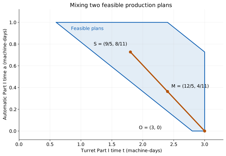
Mix two plans from Kantorovich's published machine example
Fixed published illustrative data from Kantorovich, Example 1 and Table 1, pp. 369–370: capacities (3, 3, 1) machine-days and Part I/II rates (10/20, 20/30, 30/80). Allocations S = (2, 9/5, 8/11) and O = (8/3, 3, 0) are our exact re-derivations. The model uses divisible time, full utilization, matching parts, and no setup costs. The initial midpoint and all weight changes are hypothetical mixtures, not historical observations.
Try weights $0$, $1/2$, and $1$. The dot moves along the segment; the output shows all three allocated times, both part totals, and the averaged endpoint output. The rates, capacities, and model assumptions stay fixed. Changing the weight is a hypothetical time-sharing experiment, not a historical observation. The reset restores the published-data baseline with our midpoint mixture. The exact midpoint calculation and static figure remain useful without JavaScript.
Convex sets: every segment stays inside
A set $C\subseteq\mathbb R^n$ is convex when
\[x,y\in C,\quad0\le\theta\le1 \quad\Longrightarrow\quad(1-\theta)x+\theta y\in C.\]The symbol $\in$ means “belongs to”; $\mathbb R^n$ is the space of lists of $n$ real coordinates. The points $(1-\theta)x+\theta y$ form the line segment from $x$ to $y$. The condition must hold for every pair and every allowed weight. One successful segment is an illustration; one failed segment disproves convexity. See Boyd and Vandenberghe, slide 2.3.
A convex combination of several points is $\sum_i\theta_i x_i$, with $\theta_i\ge0$ and $\sum_i\theta_i=1$. Repeated mixing shows that a convex set contains every finite convex combination of its points. The convex hull of a set is the collection of all these combinations. See slide 2.4.
Why linear constraints and intersections work
An affine expression is a linear expression plus a constant: $g(x)=b^Tx+d$, where $b^Tx=\sum_i b_ix_i$ is a dot product. It preserves weighted averages:
\[g((1-\theta)x+\theta y)=(1-\theta)g(x)+\theta g(y).\]If both endpoint values are at most a limit, so is the average. If both equal a required value, their average equals it too. Thus a linear inequality describes a convex half-space, and linear equalities describe a convex affine set. A finite intersection of such constraints is a polyhedron. See slides 2.6 and 2.9.
More generally, intersections of convex sets are convex: a segment that stays in every set stays in their intersection. This proof covers the machine model’s simultaneous capacity and balance restrictions. Unions need not work: the supplementary invented set $\lbrack-2,-1\rbrack\cup\lbrack1,2\rbrack$ contains $-1$ and $1$ but misses their midpoint $0$. See the intersection rule, slide 2.12.
A filled disk is convex; its circumference alone is not, since the midpoint of two opposite boundary points lies at the center. A single point and the empty set are convex too: there is no pair violating the definition. Convexity does not require a curved boundary, nonempty interior, or infinitely many points.
Cones and separation
A convex cone contains every nonnegative combination $\alpha x+\beta y$ of its points, where $\alpha,\beta\ge0$ need not add to one. For example, nonnegative activity levels applied to fixed production columns generate such a cone. This extends mixing by allowing the total scale to change. See slide 2.5.
Farkas’ lemma asks whether a target belongs to a finitely generated cone. If it does not, a linear measurement separates the target from every attainable output. That page proves the result, including the closedness assumption needed for its nearest-point construction.
Convex functions: compare a mixture with a mixed value
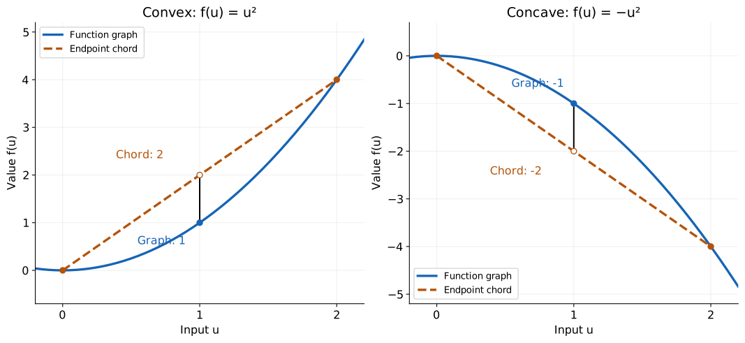
Feasibility alone does not tell us how a nonlinear cost changes when we mix inputs. For a supplementary invented illustration, suppose operating intensity $u$ has cost $f(u)=u^2$. Compare intensities 0 and 2 with equal weights:
\[f\!\left(\frac{0+2}{2}\right)=1, \qquad\frac{f(0)+f(2)}2=2.\]Operating steadily at the average intensity costs less in this model than spending half the time at each extreme. The expression on the left evaluates the average input; the right averages the two costs. They are different operations. This nonlinear cost is a teaching choice, not part of Kantorovich’s published machine data.
The chord inequality
A function $f:C\to\mathbb R$ on a convex domain $C$ is convex if
\[f((1-\theta)x+\theta y) \le(1-\theta)f(x)+\theta f(y) \quad(x,y\in C,\ 0\le\theta\le1).\]A domain is the set of allowed inputs. A chord is the straight segment joining the graph points $(x,f(x))$ and $(y,f(y))$. At a mixed input, the graph is no higher than the chord. A function is concave when the inequality reverses, equivalently when $-f$ is convex. Affine functions satisfy equality and are both convex and concave. See Boyd and Vandenberghe, slide 3.1.
For $f(u)=u^2$, subtract the left side from the right and expand:
\[\begin{aligned} &(1-\theta)x^2+\theta y^2-((1-\theta)x+\theta y)^2\\ &\qquad=\theta(1-\theta)(x-y)^2\ge0. \end{aligned}\]This original calculation proves the inequality for all real endpoints. It also explains when equality holds: at either endpoint weight, or when $x=y$. For $-u^2$ the difference has the opposite sign, so that function is concave and fails the convex inequality whenever the endpoints differ and $0<\theta<1$.
Compare the cost of a mixed input with the average cost
Supplementary invented teaching examples, without physical units. Blue is the function graph; dashed orange is the endpoint chord. The difference of their heights at the mixed input tests that particular chord.
Change the endpoints and weight, then compare $u^2$, $\lvert u\rvert$ (absolute value), and $-u^2$. Equal endpoints collapse the chord to one point; weights 0 and 1 give equality. Absolute value has a corner at zero, but still satisfies the inequality. These are supplementary invented teaching examples. The controls test particular chords; the algebra above proves the all-endpoints claim for the square.
Averaging more inputs: Jensen’s inequality
Repeated use of the two-point definition gives the finite weighted form of Jensen’s inequality:
\[f\!\left(\sum_i\theta_i x_i\right)\le\sum_i\theta_i f(x_i), \qquad\theta_i\ge0,\quad\sum_i\theta_i=1.\]It compares a function of a weighted mean with the weighted mean of the function values. See Boyd and Vandenberghe, slide 3.13. For the supplementary inputs $0,1,2$ with equal weights and $f(u)=u^2$, it reads $1\le5/3$. It does not say that mixing beats the best endpoint: the earlier square example had $f(0)=0<f(1)=1$.
Turning function inequalities into convex feasible sets
A sublevel set is a set of inputs whose function values are below a threshold: $C_\alpha={x\in C:f(x)\le\alpha}$. If $f$ is convex, then for $x,y\in C_\alpha$,
\[f((1-\theta)x+\theta y) \le(1-\theta)\alpha+\theta\alpha=\alpha.\]Thus the sublevel set is convex. For example, $u^2\le4$ gives the interval $\lbrack-2,2\rbrack$. Equality constraints behave differently: $u^2=4$ gives just ${-2,2}$, which misses its midpoint. This is why the standard convex formulation uses convex inequalities and affine equalities. See sublevel sets, slide 3.12, and convex optimization form, slide 4.7.
The epigraph of $f$ is its graph together with all the points above it:
\[\operatorname{epi}f=\{(x,s):x\in C,\ s\ge f(x)\}.\]Here $s$ is a height coordinate. A convex function has a convex epigraph: mixing two allowed heights leaves a height at least as large as the mixed function value. Conversely, apply epigraph convexity to heights $f(x)$ and $f(y)$ to recover the chord inequality. See slide 3.12. This gives a direct bridge between convex functions and convex sets; the graph alone need not be a convex set.
Why local minima become global
Consider minimizing a convex function $f$ over a convex feasible set $C$. A local minimizer $x_\star$ is at least as good as every feasible point sufficiently close to it. A global minimizer is at least as good as every point in $C$.
Suppose a better feasible point $y$ existed, with $f(y)<f(x_\star)$. For any $0<\theta<1$, convexity of the set makes $x_\theta=(1-\theta)x_\star+\theta y$ feasible. Convexity of the function gives
\[f(x_\theta)\le(1-\theta)f(x_\star)+\theta f(y)<f(x_\star).\]Take $\theta$ arbitrarily small: the better point $x_\theta$ becomes arbitrarily close to $x_\star$, contradicting local minimality. Every local minimizer is global. Both convexities are used: one keeps the segment feasible, the other controls its objective. This is an expanded derivation of Boyd and Vandenberghe’s argument, slide 4.9.
The production model maximizes an affine output; equivalently, it minimizes its negative, which is convex. More generally, maximizing a concave function over a convex set has the same guarantee after negating the objective. The guarantee does not cover maximizing an arbitrary convex function.
Strict convexity gives at most one minimizer
A function is strictly convex if the chord inequality is strict whenever $x\ne y$ and $0<\theta<1$. See slide 3.1. If two distinct feasible minimizers had the same value, their midpoint would have a smaller value, a contradiction. Thus there is at most one minimizer on a convex feasible set.
Existence is a separate question. The supplementary function $f(u)=1/u$ on the convex domain $u>0$ has $f’‘(u)=2/u^3>0$, yet approaches zero without ever reaching it. It is strictly convex and has no minimizer. Similarly, $u^2$ on the open interval $(0,1)$ approaches its best lower bound at an excluded endpoint. These examples show why “strictly convex” must not be read as “a unique solution exists.” Compare the unattained-optimum examples, slide 4.4.
Slopes and curvature: links to quadratic forms
For a differentiable function, the gradient $\nabla f(x)$ collects the coordinate slopes; its dot product with a displacement gives the tangent approximation. On an open convex domain, convexity is equivalent to the global tangent bound
\[f(y)\ge f(x)+\nabla f(x)^T(y-x)\qquad\text{for all }x,y.\]See Boyd and Vandenberghe, slide 3.8. For our supplementary square, the tangent at $u=1$ is $1+2(u-1)=2u-1$, and $u^2-(2u-1)=(u-1)^2\ge0$. Chords bound a convex graph from above between their endpoints; tangent lines bound it from below.
If $\nabla f(x_\star)=0$, the bound proves global minimality. At a constrained boundary, the gradient need not vanish: minimizing $u^2$ over $u\ge1$ gives $u_\star=1$ and derivative 2. For a differentiable convex function defined on an open convex neighborhood of the convex feasible set, the correct constrained criterion is
\[\nabla f(x_\star)^T(y-x_\star)\ge0\qquad\text{for every feasible }y.\]Every feasible direction has nonnegative first-order change. In the boundary example, $2(y-1)\ge0$. See slide 4.10; Optimization duality expresses constrained stationarity using multipliers.
The Hessian tests every direction
The Hessian $\nabla^2 f(x)$ is the matrix of second partial derivatives. If $f$ is twice continuously differentiable on an open convex domain, then
\[f\text{ is convex}\quad\Longleftrightarrow\quad v^T\nabla^2 f(x)v\ge0\quad\text{for every }x,v.\]The matrix condition is positive semidefiniteness (PSD). Along a line $g(s)=f(x+sv)$, the second derivative is $g’‘(s)=v^T\nabla^2 f(x+sv)v$: the test checks upward curvature along every direction, everywhere in the domain. Positive definiteness everywhere is sufficient for strict convexity, but is not necessary: $u^4$ is strictly convex although its second derivative vanishes at zero. See slides 3.9–3.10. For $u^4$, the derivative $4u^3$ is strictly increasing, so every nontrivial chord has strictly larger average slope after its interior point than before it.
For a symmetric matrix $A$ and fixed vector $r$, the quadratic function
\[f(x)=\frac12x^TAx-r^Tx+d\]has gradient $Ax-r$ and Hessian $A$. Therefore PSD gives convexity; symmetric positive definiteness gives strict convexity and an invertible $A$, so this unconstrained quadratic has the unique minimizer solving $Ax=r$. PSD alone need not give existence: with $A=\operatorname{diag}(1,0)$ and $r=(0,1)^T$, the objective $x_1^2/2-x_2$ decreases without bound as $x_2$ grows. If instead $r=0$, every $(0,x_2)$ minimizes it.
Least squares supplies the recurring example $f(x)=\lVert Bx-b\rVert_2^2$, where $Bx$ is a prediction and $b$ a measurement vector. Its Hessian is $2B^TB$, and $v^T(2B^TB)v=2\lVert Bv\rVert_2^2\ge0$. It is convex even when columns of $B$ are dependent. Independent columns make that Hessian positive definite and the fit unique. The quadratic-form page develops the derivatives and normal equations.
Common mistakes and useful counterexamples
These are supplementary invented examples and deductions.
- Checking just a midpoint is not a proof. A passing test checks one pair and weight; convexity quantifies over all of them. The square-gap identity above supplies that proof for $u^2$.
- A convex domain does not make every function on it convex. $-u^2$ is not convex on $\mathbb R$. Conversely, a convex objective does not repair a nonconvex feasible set: $u^2$ on ${-1,2}$ has two isolated local minimizers, of which only $-1$ is global.
- Convex does not mean strictly curved or smooth. Affine functions are convex, and $\lvert u\rvert$ is convex with a corner. On the positive half-line, $\lvert u\rvert=u$, so it is not strictly convex there.
- Positive coordinate curvature is insufficient. $f(x_1,x_2)=x_1^2+4x_1x_2+x_2^2$ has Hessian diagonal entries 2, but along $(s,-s)$ it equals $-2s^2$. Check the full Hessian in all directions, as in the quadratic-form counterexample.
- One positive Hessian does not prove global convexity. $u^4-u^2$ has positive second derivative at $u=1$ and negative second derivative at $u=0$. The Hessian criterion applies throughout the stated domain.
- Convexity alone does not settle duality or existence. The duality page distinguishes strong duality, attainment, and constraint qualifications such as Slater’s condition.
Practice problems
These are original exercises. Try each before revealing its hint or worked solution.
1. Hand calculation: a quarter of the optimal plan
Using the published machine data, compute $x_{1/4}=(3/4)x^{\mathrm S}+(1/4)x^{\mathrm O}$. Verify the balance equation and output without rounding.
Hint
Average the times coordinate by coordinate. The output must also be the same weighted average of $856/11$ and $260/3$.
Worked solution
The times are $m=13/6$, $t=21/10$, and $a=6/11$. Each satisfies its capacity. The balance is $30m+50t+110a=65+105+60=230$. Part I output is
\[P=\frac{65}{3}+42+\frac{180}{11}=\frac{2641}{33}.\]Part II output is $Q=230-130/3-63-480/11=2641/33$. The averaged endpoint output is $(3/4)(856/11)+(1/4)(260/3)=2641/33$, about $80.03$ complete sets per day. This is a hypothetical mixture of the re-derived plans, not a value printed in the historical source.
2. Interpretation: mixing and whole-day assignments
Suppose a hypothetical new policy requires each machine to make one part for its entire working day. May we still regard every convex mixture of two allowed daily assignments as an allowed daily assignment? Would randomizing between them change the answer?
Hint
Consider the automatic machine alone: its Part I time must be either zero or one machine-day under the new policy.
Worked solution
No. The midpoint of automatic allocations 0 and 1 is $1/2$, forbidden by this hypothetical policy. The full-day assignment set is therefore not convex, even before imposing matching parts. Randomizing between full-day assignments gives a fractional expected allocation, but each realized day still uses a whole assignment; expectation does not establish daily feasibility of the fractional plan. Over several days, time averages may have an operational meaning if storage and the output requirements permit it. Those are additional assumptions. The original divisible-time model already permits splitting a day, which is why its convex mixtures are feasible directly.
3. Logical reasoning: what can the set of minimizers look like?
Prove that the set of minimizers of a convex function over a convex feasible set is convex. Does that set have to contain a point? What changes if the objective is strictly convex?
Hint
If two points attain the same best value, convexity bounds the value at their mixture from above. Optimality bounds it from below.
Worked solution
If $x,y$ both attain the minimum $p$, their feasible mixture has value at most $(1-\theta)p+\theta p=p$. It cannot be smaller than the minimum, so it also attains $p$. The minimizer set is convex. It can be empty: $1/u$ for $u>0$ never attains its lower bound zero. Under strict convexity, distinct minimizers are impossible, so the set is either empty or a singleton. Convexity describes the shape of the solution set without supplying existence.
4. Practical application: a constrained least-squares fit
A supplementary invented model predicts one measured total 3 using two nonnegative contributions $x_1,x_2$. Minimize $(x_1+x_2-3)^2$ subject to $x_1,x_2\ge0$. Is this a convex problem? Find all minimizers. What happens after adding a penalty $\alpha(x_1^2+x_2^2)$ with $\alpha>0$?
Hint
The unpenalized objective depends only on the sum. For the penalized problem, symmetry suggests equal contributions; verify using the gradient and Hessian.
Worked solution
The nonnegative quadrant is convex. The Hessian of the objective is
\[2\begin{bmatrix}1&1\\1&1\end{bmatrix},\]whose quadratic form is $2(v_1+v_2)^2\ge0$. Every nonnegative pair with $x_1+x_2=3$ has objective zero, so the minimizers are precisely the segment from $(0,3)$ to $(3,0)$.
The penalty adds $2\alpha I$ to the Hessian, where $I$ is the identity matrix. Its quadratic form becomes $2(v_1+v_2)^2+2\alpha(v_1^2+v_2^2)>0$ for nonzero $v$. Stationarity gives $x_1+x_2-3+\alpha x_1=0$ and the corresponding equation for $x_2$. Subtracting gives $x_1=x_2$; hence both equal $3/(2+\alpha)>0$. This feasible stationary point is the unique global minimizer. The penalty changes the objective: its fitted sum is now $6/(2+\alpha)<3$, so uniqueness comes with a changed fit.
References and further learning
- L. V. Kantorovich, Mathematical Methods of Organizing and Planning Production, English translation (1960) of the 1939 monograph. Example 1 and Table 1, pp. 369–370, provide the machine rates; Table 2, p. 371, gives the reported integer outputs; Problem A, pp. 371–372, states the divisible-time, full-use, matching-output formulation. Useful for seeing why a production plan is a collection of activities that can be mixed.
- Stephen Boyd and Lieven Vandenberghe, Convex Optimization: Chapter 2 slides, revised with Parth Nobel. Slides 2.3–2.5 define convex sets, hulls, and cones; 2.6–2.12 connect constraints, polyhedra, and intersections. Use these to practice recognizing convex feasible regions.
- Boyd and Vandenberghe, Chapter 3 slides. Slides 3.1, 3.8–3.13 explain chords, derivative tests, epigraphs, and Jensen’s inequality. Later slides develop rules for proving convexity without expanding every derivative.
- Boyd and Vandenberghe, Chapter 4 slides. Slides 4.4 and 4.7–4.11 distinguish unattained optima, convex formulations, local/global minima, and constrained optimality. Useful for checking exactly which assumptions justify an optimization claim.
- The authors’ book and course resource page. The freely available textbook provides longer proofs and exercises, especially Chapters 2–4. Continue with Optimization duality for bounds and multipliers, or Quadratic forms for the matrix curvature calculations.