Optimization
Optimization duality
Turn production constraints into optimality certificates, prove LP strong duality with Farkas’ lemma, and derive Lagrange duals and KKT conditions.
Kantorovich’s production problem: how can we know a plan is best?
A feasible production plan proves what a factory can achieve. It does not prove that another allocation could not achieve more. Optimization duality addresses this second question by constructing a related optimization problem whose feasible solutions certify bounds on the original objective. The original problem is the primal; the bounding problem is its dual. For the LP version of this idea, see MIT’s duality notes, “Duality”.
The Linear programming page derives and solves Kantorovich’s machine-allocation example. Here we keep its published rates and ask a different question: how should we choose the weights that certify the answer? Later, Farkas’ lemma will explain why such a certificate must exist for a feasible LP with a finite optimum.
Kantorovich’s 1939 monograph opens with an illustrative metalworking problem. Each completed item needs one Part I and one Part II. These are his Example 1 and Table 1 data, not observations from an actual factory. See pp. 369–370 of the English translation.
| Machine group | Available machine-days | Part I per machine-day | Part II per machine-day |
|---|---|---|---|
| Milling | 3 | 10 | 20 |
| Turret | 3 | 20 | 30 |
| Automatic turret | 1 | 30 | 80 |
The algebra below is our modern re-derivation. Time is divisible, rates are constant and additive, all available time is used, and there are no setup costs. We require exactly matching part totals. A fractional output means a daily production rate, not a whole-item schedule. The source’s Table 2 reports integer totals of 86 for its specialized plan; our exact continuous calculation from Table 1 gives $260/3$.
Let $m,t,a$ be machine-days making Part I. The remaining times make Part II, so
\[P=10m+20t+30a,\qquad Q=230-20m-30t-80a,\] \[0\le m,t\le3,\qquad 0\le a\le1,\qquad P=Q=z.\]The primal maximizes $z$. At $(m,t,a)=(8/3,3,0)$,
\[P=10(8/3)+60=260/3,\qquad Q=230-20(8/3)-90=260/3.\]This is evidence that the optimum is at least $260/3$. To prove equality, we need an upper bound that applies to every feasible allocation.
Price the parts instead of searching over plans
Choose a weight $\theta$ for Part I and $1-\theta$ for Part II. For now, take $0\le\theta\le1$. Matching output gives
\[z=\theta P+(1-\theta)Q.\]These weights are certificate coefficients, not market prices. Each milling machine-day contributes either $10\theta$ or $20(1-\theta)$ to weighted output, or an average of them if its time is split. Its contribution cannot exceed the larger number. The same argument for each group gives
\[\begin{aligned} z\le U(\theta) ={}&3\max\lbrace 10\theta,20(1-\theta)\rbrace \\ &+3\max\lbrace 20\theta,30(1-\theta)\rbrace \\ &+\max\lbrace 30\theta,80(1-\theta)\rbrace . \end{aligned}\]The factors $3,3,1$ are available machine-days; $U$ measures complete sets per day. Every choice of weight gives a bound. Dual optimization searches for the smallest bound. Kantorovich’s Appendix I develops his resolving multipliers; our one-parameter calculation is a modern way to expose their bounding role. See Appendix I, §§1–3.
At $\theta=1/2$, the three largest weighted rates are $10,15,40$, so $U(1/2)=115$. This is valid but inconclusive: it leaves room between the achieved $86.67$ and the certified upper bound $115$.
The milling group switches its preferred part where
\[10\theta=20(1-\theta)\quad\Longrightarrow\quad\theta=2/3.\]At that weight,
\[U(2/3)=3(20/3)+3(40/3)+80/3=260/3.\]The feasible plan and the bound meet. We have proved optimality without comparing that plan with every other plan.
See the bound tighten
The turret and automatic groups switch at $\theta=3/5$ and $8/11$. Substituting the larger rate on each interval gives our exact piecewise formula:
\[U(\theta)= \begin{cases} 230(1-\theta),&0\le\theta\le3/5,\\ 140-80\theta,&3/5\le\theta\le2/3,\\ 80+10\theta,&2/3\le\theta\le8/11,\\ 120\theta,&8/11\le\theta\le1. \end{cases}\]It decreases up to $2/3$ and increases afterward. Thus $2/3$ minimizes this family of bounds. The corners occur when a machine group becomes indifferent between its two parts.
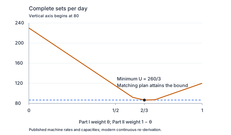
Choose the weights of a production certificate
Published illustrative-data baseline from Kantorovich, Example 1 and Table 1, pp. 369–370: capacities (3, 3, 1) machine-days and Part I/II rates (10/20, 20/30, 30/80). Data remain fixed. The modern model uses divisible time, full utilization, exactly matching parts, and no setup costs. The initial weight 2/3 is our derived certificate; changing it is a hypothetical certificate experiment.
Try $0$, $1/2$, $2/3$, and $1$. The original machine capacities and rates stay fixed; changing the weight is a hypothetical certificate experiment, not new historical data. “Restore published-data baseline” restores those fixed data with our derived weight $2/3$. Keyboard users can type a weight or activate either button. The piecewise formula, figure, and calculations above remain usable without JavaScript.
Recover the full dual rather than only a family of weights
Let $h_{jk}\ge0$ be time assigned to part $k$ in group $j$, with capacity $N_j$ and rate $r_{jk}$. The historical model imposes
\[h_{j1}+h_{j2}=N_j,\qquad \sum_j r_{jk}h_{jk}=z\quad(k=1,2).\]Use part weights $\lambda_1+\lambda_2=1$ and machine values $w_j\ge r_{jk}\lambda_k$. Then
\[z=\sum_{j,k}\lambda_k r_{jk}h_{jk} \le\sum_{j,k}w_jh_{jk}=\sum_jN_jw_j.\]The full dual minimizes $\sum_jN_jw_j$ under those inequalities and the normalization. Both $\lambda_k$ and $w_j$ are unrestricted in sign: their primal constraints are equalities. For fixed $\lambda=(\theta,1-\theta)$, minimizing over $w_j$ selects the maxima in $U(\theta)$. The lab explores only $\theta\in[0,1]$, a subset of the full dual’s allowable weights. This subset contains a matching certificate, which already proves optimality for the full pair. See the LP page’s complete historical dual.
Construct an LP dual by deciding which inequalities preserve a bound
Consider the resource model
\[\begin{aligned} \text{maximize}\quad &c^Tx\\ \text{subject to}\quad &Ax\le b,\quad x\ge0. \end{aligned}\]Here $x\in\mathbb R^n$ contains activity levels, $A\in\mathbb R^{r\times n}$ contains resource consumption, $b\in\mathbb R^r$ contains capacities, and $c\in\mathbb R^n$ contains profit per activity. The transpose $A^T$ exchanges rows and columns, so $(A^Ty)_j$ is the weighted input requirement of activity $j$.
Choose $y\ge0$ so that multiplying the resource inequalities preserves their direction. If also $A^Ty\ge c$, then for every primal feasible $x$,
\[c^Tx\le x^TA^Ty=y^TAx\le y^Tb.\]The first inequality uses $x\ge0$; the last uses $y\ge0$. Therefore the smallest upper bound of this form comes from
\[\begin{aligned} \text{minimize}\quad &b^Ty\\ \text{subject to}\quad &A^Ty\ge c,\quad y\ge0. \end{aligned}\]This inequality is weak duality. It explains the transpose, the multiplier signs, and the reversed optimization direction together. See MIT’s notes, “Duality” and “Rules for Taking Duals”.
Sign rules are consequences of the bound
For a maximization primal and a minimization dual, the correspondence is:
| Primal feature | Corresponding dual requirement |
|---|---|
| Row $a_i^Tx\le b_i$ | $y_i\ge0$ |
| Row $a_i^Tx\ge b_i$ | $y_i\le0$ |
| Row $a_i^Tx=b_i$ | $y_i$ unrestricted |
| Variable $x_j\ge0$ | $(A^Ty)_j\ge c_j$ |
| Variable $x_j\le0$ | $(A^Ty)_j\le c_j$ |
| Variable $x_j$ unrestricted | $(A^Ty)_j=c_j$ |
An equality can be multiplied by either sign. An unrestricted activity needs exact coefficient matching because either sign of $x_j$ must preserve the bound. These rules use the convention $c^Tx\le b^Ty$; changing the primal to minimization changes the rules. The historical full-use model and the resource-upper-limit model therefore have different multiplier signs without any contradiction.
As an original sign-check example, maximize $x_1+2x_2$ subject to $x_1+x_2=3$, $x_1\ge0$, with $x_2$ unrestricted. Its dual minimizes $3y$ with $y\ge1$ from $x_1$, and $y=2$ from $x_2$. Thus $y=2$ certifies value $6$, attained at $(x_1,x_2)=(0,3)$. Forcing equality multipliers to be nonnegative in general would discard valid certificates; omitting the dual equality for $x_2$ would allow invalid ones.
Why LP bounds can meet: a proof through Farkas’ lemma
LP strong duality: if the resource primal is feasible and its optimal value is finite, both the primal and its dual attain the same value. Weak duality alone does not prove existence, attainment, or equality. See MIT’s strong-duality discussion. The following is our proof, using the closed-cone and alternative results developed on the Farkas’ lemma page.
First establish that the best primal value is attained
Write $v=\sup\lbrace c^Tx:Ax\le b,\ x\ge0\rbrace $, assumed finite. A supremum is the least upper bound; it need not generally be achieved. Introduce the set
\[K=\left\lbrace \begin{bmatrix}Ax+s\\c^Tx-t\end{bmatrix}:x\ge0,\ s\ge0,\ t\ge0\right\rbrace .\]Here $s$ is unused capacity and $t$ is a nonnegative subtraction from profit. This is a cone generated by finitely many vectors: the columns $(A_j,c_j)$, the vectors $(e_i,0)$, and $(0,-1)$. The vector $e_i$ has a 1 in coordinate $i$ and zeros elsewhere. A finitely generated cone is closed, meaning that it contains limits of convergent sequences of its points. See Bertsekas, “Farkas–Minkowski–Weyl Theorems,” part (a), PDF p. 105.
Choose feasible $x^{(k)}$ with $c^Tx^{(k)}\to v$. Then $(b,c^Tx^{(k)})\in K$, using $s=b-Ax^{(k)}$ and $t=0$. Closedness gives $(b,v)\in K$. Consequently some nonnegative $x,s,t$ satisfy
\[Ax+s=b,\qquad c^Tx-t=v.\]The first equation makes $x$ feasible; the second gives $c^Tx\ge v$. Since $v$ is already an upper bound, $c^Tx=v$ and $t=0$. This proves primal attainment even if the feasible points in the approximating sequence themselves escape to infinity.
Then establish that a dual certificate attains the same value
For unrestricted variables $x$, combine $Ax\le b$ and $-x\le0$ as $Gx\le h$, with
\[G=\begin{bmatrix}A\\-I\end{bmatrix},\qquad h=\begin{bmatrix}b\\0\end{bmatrix}.\]We claim that any valid upper bound $c^Tx\le v$ on this nonempty system admits $\mu\ge0$ with $G^T\mu=c$ and $h^T\mu\le v$. To prove it using the equality form of Farkas’ lemma, consider
\[\begin{bmatrix}G^T&0\\h^T&1\end{bmatrix} \begin{bmatrix}\mu\\\rho\end{bmatrix} =\begin{bmatrix}c\\v\end{bmatrix},\qquad \mu\ge0,\quad\rho\ge0.\]If this system had no solution, Farkas would provide $(u,\alpha)$ such that
\[Gu+\alpha h\ge0,\qquad\alpha\ge0,\qquad c^Tu+\alpha v<0.\]If $\alpha>0$, the point $x=-u/\alpha$ would satisfy $Gx\le h$ and $c^Tx>v$, contradicting the bound. If $\alpha=0$, choose any feasible $x_0$. Then $x_0-\tau u$ stays feasible for every $\tau\ge0$, while its objective tends to $+\infty$ because $c^Tu<0$. This also contradicts the bound. Therefore $\mu,\rho$ exist. This argument uses the equality alternative; see also Farina, Theorem L6.1, for the inequality alternative.
Partition $\mu=(y,s)$ according to the rows of $A$ and $-I$. Its equations give
\[A^Ty-s=c,\quad y,s\ge0,\quad b^Ty+\rho=v.\]Thus $y$ is dual feasible and $b^Ty\le v$. Weak duality applied to the attained primal optimum gives $v\le b^Ty$. Both inequalities force $b^Ty=v$.
Farkas supplies the bound coefficients, while finite-cone closedness supplies primal attainment. Both ingredients matter; ruling out every strictly better target alone would not explain why the primal optimum is achieved.
Complementary slackness: locate every possible loss in the certificate
For feasible $x,y$ in the resource pair, subtract the earned profit from its bound:
\[b^Ty-c^Tx=y^T(b-Ax)+x^T(A^Ty-c).\]The duality gap of this feasible pair is the left side. Every term on the right is nonnegative. Consequently the gap is zero exactly when
\[y_i\bigl(b_i-(Ax)_i\bigr)=0\quad\text{for every }i,\] \[x_j\bigl((A^Ty)_j-c_j\bigr)=0\quad\text{for every }j.\]These are complementary slackness conditions: a positive resource price requires all that resource to be used, and a positive activity requires its priced inputs to equal its profit. Together with primal and dual feasibility they characterize optimal pairs for this LP. See MIT’s notes, “Complementary Slackness”.
For the historical full-use model, the same subtraction takes a slightly different form:
\[\sum_jN_jw_j-z=\sum_{j,k}h_{jk}\bigl(w_j-r_{jk}\lambda_k\bigr).\]At $\lambda=(2/3,1/3)$, both milling rates equal $w_M=20/3$, so milling may split its time. Turret Part II has strictly smaller weighted output than Part I, and automatic Part I has strictly smaller weighted output than Part II. Equality of the certificate therefore forces those inferior activities to have zero time. The mixed milling allocation is then determined by matching the two part totals.
A constraint being tight does not force its price to be positive. In the supplementary LP $\max x_1$ with $0\le x_1,x_2\le1$, the point $(1,1)$ binds both upper limits, but the optimal resource prices are $(1,0)$.
From weighted linear constraints to a Lagrangian
The machine proof constructed bounds by weighting constraints. The same construction works when the objective or restrictions are nonlinear. We now use the standard minimization convention, so dual certificates will be lower bounds.
Write a general problem as
\[p^{\star}=\inf_{x\in X}\lbrace f_0(x):f_i(x)\le0\ (i=1,\ldots,r),\ h_j(x)=0\ (j=1,\ldots,q)\rbrace .\]The set $X$ is the domain kept explicitly, such as $\mathbb R^n$, nonnegative vectors, or even binary choices. A function $f_i$ measures a constraint’s signed violation; $f_i(x)\le0$ means it is satisfied. The Lagrangian puts these functions into the objective:
\[L(x,\lambda,\nu)=f_0(x)+\sum_i\lambda_i f_i(x)+\sum_j\nu_jh_j(x),\qquad\lambda\ge0.\]The coefficients $\lambda_i,\nu_j$ are Lagrange multipliers. Equality multipliers $\nu_j$ are unrestricted. Define the dual function
\[g(\lambda,\nu)=\inf_{x\in X}L(x,\lambda,\nu).\]The constraints incorporated into $L$ are removed from this inner minimization; restrictions retained in $X$ remain. For every primal feasible $x$,
\[g(\lambda,\nu)\le L(x,\lambda,\nu)\le f_0(x).\]The second inequality follows from $\lambda_i f_i(x)\le0$ and $h_j(x)=0$. Thus the Lagrange dual problem maximizes $g(\lambda,\nu)$ over $\lambda\ge0$ and unrestricted $\nu$. Its supremum $d^{\star}$ satisfies $d^{\star}\le p^{\star}$. The inner infimum can be $-\infty$; such multipliers give no useful finite bound. These definitions and the bound construction follow Boyd and Vandenberghe’s duality slides, slides 5.2–5.3 and 5.10.
Our bounds also show why $g$ is concave in its multipliers: it lies at or above the line segment between any two of its finite values. For each fixed $x$, $L$ is affine in $(\lambda,\nu)$; taking the infimum gives
\[g(\eta z_1+(1-\eta)z_2)\ge\eta g(z_1)+(1-\eta)g(z_2),\qquad0\le\eta\le1,\]where $z$ collects the multipliers. This does not require the original functions to be convex. It also does not guarantee that the best dual bound equals the primal value.
Recover the resource LP without memorizing a sign table
Negate profit to minimize $-c^Tx$, keep $X=\lbrace x:x\ge0\rbrace $, and dualize $Ax-b\le0$:
\[L(x,y)=-c^Tx+y^T(Ax-b)=-b^Ty+(A^Ty-c)^Tx.\]If any coefficient of $x$ is negative, sending that nonnegative coordinate to infinity gives $g(y)=-\infty$. Otherwise the minimum is attained at $x=0$, so
\[g(y)=\begin{cases}-b^Ty,&A^Ty\ge c,\\-\infty,&\text{otherwise}. \end{cases}\]Maximizing $-b^Ty$ gives the same multipliers as minimizing $b^Ty$. The constraint $A^Ty\ge c$ emerges from asking when the inner minimization has a finite value. The objective value is negated because we first negated the primal profit.
When do nonlinear bounds meet?
A function is convex if its value along a segment is no greater than the corresponding average of endpoint values. For a convex optimization problem, $X$ is convex, $f_0$ and the $f_i$ are convex, and the $h_j$ are affine. Convexity develops these set and function definitions, the local-to-global minimum proof, and derivative tests. Convexity alone does not supply every existence and multiplier guarantee.
A useful sufficient condition is Slater’s condition: when $X=\mathbb R^n$ and these functions are finite everywhere, there exists a point $\bar x$ with $f_i(\bar x)<0$ for every inequality and $h_j(\bar x)=0$ for every equality. If the primal value is finite, this condition guarantees $d^{\star}=p^{\star}$ and attainment of the dual optimum. It does not by itself guarantee primal attainment. More general domain versions use relative interiors. See Boyd and Vandenberghe, slide 5.13.
Supplementary convex example: derive both solutions
This is an invented teaching example, not historical data:
\[\text{minimize }(x-2)^2\quad\text{subject to }x\le1,\qquad x\in\mathbb R.\]The unconstrained minimum at $x=2$ is forbidden. Among $x\le1$, the nearest point to 2 is $x^{\star}=1$, with $p^{\star}=1$. The strictly feasible point $x=0$ verifies Slater’s condition.
Form the Lagrangian and complete the square:
\[\begin{aligned} L(x,\lambda)&=(x-2)^2+\lambda(x-1)\\ &=(x-2+\lambda/2)^2+\lambda-\lambda^2/4. \end{aligned}\]For fixed $\lambda\ge0$, the inner minimizer is $x=2-\lambda/2$, which is allowed to violate $x\le1$. Therefore
\[g(\lambda)=\lambda-\lambda^2/4=1-(\lambda-2)^2/4.\]The dual maximum is $1$ at $\lambda^{\star}=2$. The primal and dual values meet, and the inner minimizer at that multiplier is the feasible point $x=1$.
KKT conditions explain the matching point
For differentiable functions with $X=\mathbb R^n$, the Karush–Kuhn–Tucker (KKT) conditions combine feasibility, complementary slackness, and stationarity:
\[\begin{aligned} &f_i(x^{\star})\le0,\qquad h_j(x^{\star})=0,\\ &\lambda_i^{\star}\ge0,\qquad\lambda_i^{\star}f_i(x^{\star})=0,\\ &\nabla f_0(x^{\star})+\sum_i\lambda_i^{\star}\nabla f_i(x^{\star}) +\sum_j\nu_j^{\star}\nabla h_j(x^{\star})=0. \end{aligned}\]The gradient $\nabla f$ collects first derivatives; stationarity says that the Lagrangian has zero first derivative in every direction. For a convex problem, these conditions suffice for global optimality: stationarity minimizes the convex Lagrangian, and complementary slackness makes that minimum equal the primal objective. With Slater’s condition, every attained primal optimum has multipliers satisfying KKT. In a nonconvex problem, stationarity alone need not minimize the Lagrangian globally. See Boyd and Vandenberghe, PDF pp. 22–23.
In our example, stationarity is $2(x-2)+\lambda=0$ and complementary slackness is $\lambda(x-1)=0$. The branch $\lambda=0$ would force the infeasible point $x=2$. Hence $x=1$ and $\lambda=2$, agreeing with the direct calculations.
A positive gap: binary decisions leave a bound unattained by any plan
Here is a second supplementary invented example:
\[\text{minimize }-x\quad\text{subject to }x\le1/2,\qquad x\in\lbrace 0,1\rbrace .\]Only $x=0$ is feasible, so $p^{\star}=0$. Keep the binary domain in the inner minimization and dualize the inequality:
\[g(\lambda)=\min\lbrace -\lambda/2,-1+\lambda/2\rbrace ,\qquad\lambda\ge0.\]The two affine expressions intersect at $\lambda=1$, where $g=-1/2$. Before this point the second is smaller and increasing; afterward the first is smaller and decreasing. Thus $d^{\star}=-1/2$ and the optimal duality gap is $p^{\star}-d^{\star}=1/2$.
Allowing $0\le x\le1$ is a continuous relaxation: it admits additional choices. That relaxation attains $-1/2$ at $x=1/2$, but no feasible binary plan does. This directly verifies a limitation of this dual construction. It does not claim that every nonconvex problem has a positive gap, or that a different formulation must have the same dual.
Multipliers measure the value of relaxing a requirement
For the maximization resource LP, define $V(b)$ as the optimal profit at capacities $b$. If $y^{\star}$ is optimal at $b$, it remains dual feasible when only $b$ changes. Thus
\[V(b+\Delta b)\le(b+\Delta b)^Ty^{\star}=V(b)+(y^{\star})^T\Delta b.\]This is an upper bound, not an unconditional prediction. Equality requires a plan that reaches the changed bound. The historical machine sensitivity calculation finds precisely when the old automatic-time price $80/3$ is attainable: adding $\delta$ machine-days requires $m=8/3+(8/3)\delta\le3$, so the old specialization works only through $\delta=1/8$.
For the minimization convention, relaxing $f_i(x)\le0$ to $f_i(x)\le u_i$ changes the dual bound to $g(\lambda,\nu)-\lambda^Tu$. At an attained dual optimum with strong duality,
\[p(u)\ge p(0)-(\lambda^{\star})^Tu.\]If this value function is differentiable at zero, its derivative is $-\lambda^{\star}$. See Boyd and Vandenberghe, slides 5.23–5.25. In the convex quadratic example, the changed restriction is $x\le1+u$. For $u\le1$, the optimum is $(1-u)^2$; for $u\ge1$, it is zero. Its derivative at $u=0$ is $-2$, matching $\lambda^{\star}=2$. The bound $1-2u$ is tangent there, but the exact value contains the additional term $u^2$ until the constraint ceases to bind.
Practice problems
These exercises and their solutions are original. The first two use Kantorovich’s published rates; the remaining numerical models are supplementary teaching examples.
1. Hand calculation: check a nonoptimal certificate
Use $\theta=3/5$ in the historical machine model. Find the three $w_j$, the upper bound, and its gap above the verified plan. Which groups tie between parts?
Hint
Compute the two weighted rates in each row, then take the larger one. Multiply by available machine-days only afterward.
Worked solution
Milling has rates $6,8$, turret has $12,12$, and automatic has $18,32$. Thus $w=(8,12,32)$ and $U=3(8)+3(12)+32=92$. The gap is $92-260/3=16/3$ complete sets per day. Only turret ties. A tie makes mixing compatible with this certificate; it does not establish that the certificate is optimal.
2. Interpretation: does a feasible dual recover a production plan?
A planner chooses $\theta=1$ and tells every group to make whichever part has the larger weighted rate. Does this solve the original matching problem? What does the certificate actually prove?
Hint
Compare the selected Part I and Part II totals. Remember that the maximization used inside $U$ removed the matching requirement.
Worked solution
Every group makes Part I, giving $P=120$ and $Q=0$. This fails $P=Q$. The value $U(1)=120$ is still a valid upper bound on matching output, but the independent machine choices attaining that relaxed value are not a primal feasible plan. At the optimal weight, milling’s tie permits time to be split so that the part totals agree.
3. Logical reasoning: can strong duality hold without a dual optimizer?
Consider $\min x$ subject to $x^2\le0$, with $x\in\mathbb R$. Find its primal value and dual function. Does Slater hold? Is there a finite optimal multiplier or a KKT pair?
Hint
For $\lambda>0$, complete the square in $x+\lambda x^2$. Treat $\lambda=0$ separately.
Worked solution
Only $x=0$ is feasible, so $p^{\star}=0$. For $\lambda>0$,
\[x+\lambda x^2=\lambda\left(x+\frac1{2\lambda}\right)^2-\frac1{4\lambda},\]so $g(\lambda)=-1/(4\lambda)$; $g(0)=-\infty$. Its supremum is zero as $\lambda\to\infty$, but no finite multiplier attains it. Thus $d^{\star}=p^{\star}=0$ without dual attainment. Slater fails because $x^2<0$ is impossible. Stationarity at the only feasible point would require $1+2\lambda(0)=0$, also impossible. Failure of Slater therefore does not prove a positive gap; it removes a sufficient guarantee.
4. Practical application: value a resource requirement
Two divisible activities $a,b\ge0$ provide $2a+b$ units of service. Their total quadratic effort is $a^2+b^2$. Minimize effort while supplying at least $q>0$ service units. Derive a dual, recover the optimal allocation, and interpret the multiplier as the marginal effort of increasing demand.
Hint
Use $q-2a-b\le0$ and retain $a,b\ge0$ in the domain. Minimize $a^2+b^2+\lambda(q-2a-b)$ for fixed $\lambda\ge0$.
Worked solution
The inner minimizers are $a=\lambda$, $b=\lambda/2$, both nonnegative. Substitution gives $g(\lambda)=q\lambda-5\lambda^2/4$. Its maximum occurs at $\lambda^{\star}=2q/5$, so $a^{\star}=2q/5$, $b^{\star}=q/5$. They supply exactly $q$ and cost $q^2/5$, equal to the dual value. Differentiating that value with respect to demand gives $2q/5=\lambda^{\star}$. Increasing demand tightens the requirement, hence the positive marginal cost. At $q=5$, the allocation is $(2,1)$, the cost is $5$, and the marginal effort is $2$ per additional service unit.
References and further learning
- L. V. Kantorovich, Mathematical Methods of Organizing and Planning Production (1939; English translation, 1960): Example 1 and Table 1, pp. 369–370, supply the published illustrative machine data; Appendix I develops resolving multipliers. Our exact fractional calculations and bound curve are modern re-derivations.
- MIT 6.854, LP Duality: learn how weighted constraints give objective bounds, how variable signs determine dual constraints, and how complementary slackness certifies optimality.
- Gabriele Farina, MIT 6.7220/15.084, Lecture 6, Separation as a proof system (2025), §L6.2: study the alternative between linear feasibility and a contradiction certificate.
- Dimitri Bertsekas, Convex Analysis and Optimization slides, “Farkas–Minkowski–Weyl Theorems,” PDF p. 105: the finite-cone closedness result used to justify LP attainment.
- Stephen Boyd and Lieven Vandenberghe, Convex Optimization, Chapter 5 slides, revised with Parth Nobel: continue from Lagrangians to dual functions, Slater’s condition, KKT conditions, and sensitivity. The references above use printed slide numbers where given; PDF page anchors account for the opening pages.
- Linear programming: return to model construction, feasible geometry, simplex exchanges, and the full machine-capacity calculation.
- Farkas’ lemma: work through contradiction certificates and the cone geometry behind the strong-duality proof.