Carathéodory’s Theorem

The problem: how many points does an average need?

A mixture may involve hundreds of points even when its average has only two coordinates. Carathéodory’s theorem says that the same average can then be made from at most three of those points, with new nonnegative weights. In $\mathbb R^d$, the bound is $d+1$. This page concerns the convex hull theorem; other theorems named after Carathéodory address different questions. For the modern statement, see Bertsekas, Convex Optimization Theory, §1.2, Proposition 1.2.1.

A convex combination is a finite weighted average: the weights are nonnegative and add to one. The convex hull $\operatorname{conv}(S)$ is the set of all such averages of points in $S$. Review Convexity for why line segments and mixtures belong together.

Fourier coefficients become a geometric problem

Carathéodory’s 1911 paper studies which coefficients can occur in positive harmonic functions on a disc. A harmonic function satisfies Laplace’s equation; here it is enough to think of a smooth field constrained by its boundary behavior. His normalization and coefficient curve are

The question becomes one about the convex hull of this curve. The original introduction gives this setup; §I.9 derives a bound of dimension plus one using centers of mass. We checked these passages through Nicholas J. Williams’ English translation, introduction and §I.9 (original pp. 193–195, 200–201); the publisher’s record verifies the publication. The development below uses modern notation and calculations, rather than reproducing the historical proof. The source supplies a symbolic problem, not a numerical dataset; our chosen numerical weights are explicitly supplementary.

Why do averages appear? Consider the following modern construction. For each angle $\phi$, define a positive function using the geometric-series identity:

The denominator is positive when $r<1$. Expanding $\cos(k\theta-k\phi)$ gives coefficients $a_k=\cos k\phi$ and $b_k=\sin k\phi$. Mixing these functions with weights $\lambda_i\ge0$, $\sum_i\lambda_i=1$, preserves positivity and the constant $1/2$. Its first $2n$ coefficients are

Thus the geometric question is concrete: can we preserve these coefficients using fewer component functions? The general theorem will give at most $2n+1$ angles for any such finite mixture. It preserves the first $2n$ coefficients, not necessarily the entire function: higher coefficients may change. We use the historical coefficient curve, without claiming this general bound is the strongest bound for that special curve.

Work out the first coefficient pair

For $n=1$, the curve is the unit circle. Write a desired coefficient pair as $q=\rho(\cos\alpha,\sin\alpha)$ with $0\le\rho\le1$. Direct calculation gives

The weights sum to one; opposite circle points subtract to give radius $\rho$. At $\rho=0$ they are equal; at $\rho=1$ the second weight vanishes. This original derivation constructs a positive function for every pair in the closed unit disc using at most two angles. The general planar bound of three is sufficient but need not be attained. Access to the whole circle matters: if only a finite list of angles is allowed, those two angles may be unavailable.

Also, a pair in this disc does not make the truncated expression $1/2+r(a_1\cos\theta+b_1\sin\theta)$ positive by itself. For $(a_1,b_1)=(1,0)$ it is negative at $r=3/4$, $\theta=\pi$. The positive function constructed above retains its higher terms.

Remove one weight without moving the point

Here is a supplementary invented numerical example on the historical $n=1$ curve. Restrict the available angles to $0,\pi/2,\pi,3\pi/2$, giving

Start with the chosen weights

The opposite pairs have the same midpoint, so $A-B+C-D=0$. The coefficients $(1,-1,1,-1)$ also sum to zero. Subtract $t$ times this relation from the weights:

The weight sum and $q$ remain unchanged. To keep every weight nonnegative while increasing $t$ from zero, stop at the first weight that reaches zero:

Check both coordinates: $q_x=1/4$ and $q_y=1/2-1/4=1/4$. Four supporting points have become three. Continuing beyond $t_*$ would make the weight of $C$ negative and cease to be a convex combination.

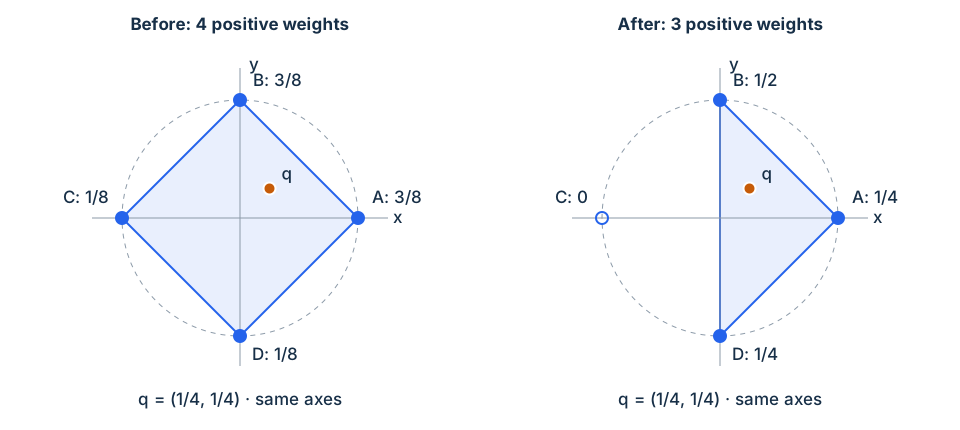
Explore the weight transfer

The circle and four angles stay fixed. The input masses are normalized to weights; they have no physical units. The slider moves from the input weights to the first zero weight along $(1,-1,1,-1)$. Changing masses creates hypothetical examples; Restore illustrative weights returns to $(3,3,1,1)$ and zero progress. Try equal masses: two weights disappear together. Try a zero mass: the input already uses at most three points. An all-zero input has no weighted average and is rejected. The calculations and static figure above remain available without JavaScript.

The theorem and its constructive proof

Let $S\subseteq\mathbb R^d$ be nonempty and $q\in\operatorname{conv}(S)$. Then there are $p_1,\ldots,p_r\in S$ and weights such that

The set $S$ may be infinite, nonconvex, or nonclosed. Membership in its convex hull already supplies a finite combination. The statement and the related cone version appear in Bertsekas, Proposition 1.2.1 and its proof, pp. 20–22. Here is an expanded weight-elimination argument.

Find an affine dependence

Start from any finite representation and discard zero weights. Suppose $m>d+1$ positive weights remain. Attach a final coordinate of one to each point:

There are more columns than coordinates, so these columns are linearly dependent. A nonzero vector $\alpha$ therefore satisfies

This is an affine dependence: moving the weights in this direction preserves both the represented point and the weight sum. Because $\alpha$ is nonzero and sums to zero, it has both positive and negative entries. The extra coordinate is what distinguishes an affine dependence from an arbitrary linear relation among the original points.

Move to the first zero weight

Set

For $\alpha_i>0$, the minimum prevents a negative new weight; for $\alpha_i\le0$, the weight cannot decrease. At least one weight becomes zero. Moreover,

Delete zero weights and repeat. Each step removes at least one point, so a representation initially using $m$ points needs at most $m-d-1$ steps when $m>d+1$. Once at most $d+1$ remain, the theorem is proved. One may continue if those remaining points are still affinely dependent; an affinely independent support is a simplex (a point, segment, triangle, tetrahedron, and their higher-dimensional counterparts).

For a numerical implementation, find a null vector of the matrix whose columns are $\widetilde p_i$, for example using QR factorization. Near dependence needs a rank tolerance; check nonnegativity, the weight sum, and the residual $|\sum_i\lambda_i p_i-q|$ after reduction. The proof gives exact identities; floating-point arithmetic gives approximate checks.

What the bound does and does not mean

Affine dimension is the relevant dimension

The affine hull is the smallest translated linear subspace containing $S$. If its dimension is $k<d$, use coordinates within that subspace: the same proof gives $k+1$ points. A set on a line in $\mathbb R^{100}$ therefore needs at most two. The circle, despite having one angle parameter, has a two-dimensional affine hull; the theorem’s general bound there is three. Its two-point formula above is a special improvement, not a calculation of affine dimension.

The bound can be necessary

For the supplementary example $S={0,e_1,\ldots,e_d}$, where $e_j$ has coordinate one in position $j$ and zero elsewhere, take

Each coordinate forces the weight of its $e_j$ to be $1/(d+1)$; the sum-to-one condition forces the same weight on $0$. Every one of these $d+1$ points is needed. Thus no smaller bound works for all sets in $\mathbb R^d$.

Existence does not imply uniqueness or an arbitrary choice

For $S={A,B,C,D}$ above, the origin is both $(A+C)/2$ and $(B+D)/2$. Conversely, the chosen $q=(1/4,1/4)$ is outside triangle $ACD$, whose points have second coordinate at most zero. The theorem promises a suitable subset, not that every subset of size three will work. Inside one fixed affinely independent simplex, the weights are unique; choosing the simplex need not be.

Convex hull and closed convex hull differ

Let $S={1,1/2,1/3,\ldots}\subset\mathbb R$. Every finite convex combination is strictly positive, although these points approach zero. Hence $0$ is in the closed convex hull, which also contains limits, but not in $\operatorname{conv}(S)$. The theorem supplies no finite representation for it. This is an original counterexample illustrating why the exact membership assumption matters.

Applications: preserve measurements with a smaller mixture

Suppose item $i$ has a feature vector $v_i\in\mathbb R^k$, and a finite probability distribution gives weights $w_i\ge0$ summing to one. Its expected features are $\mu=\sum_iw_iv_i$. Applying the theorem to the feature vectors yields a distribution on at most $k+1$ of the original items with exactly the same expected features. This is a direct corollary, not a statement that the two distributions agree in every respect.

For example, preserving $E[X]$ and $E[X^2]$ uses $v_i=(x_i,x_i^2)$, so at most three original values suffice. Preserving only $E[X]$ needs at most two but may change variance. If a cost must also remain unchanged, add it as another feature and reassess the dimension. Similarly, a time-sharing schedule can preserve a vector of average outputs with fewer operating modes, provided outputs mix linearly and there are no additional switching constraints.

The cone version replaces convex weights by nonnegative coefficients without the sum-to-one condition. In $\mathbb R^d$, a nonzero point in a generated cone needs at most $d$ generators, because ordinary linear dependence is enough. See Bertsekas, Proposition 1.2.1(a), and Farkas’ Lemma for how nonnegative combinations describe attainable targets. The additional normalization equation explains the convex bound’s extra point.

Practice

These exercises and solutions are original teaching examples.

1. Hand calculation: a weight vanishes

For $A,B,C,D$ above, use weights $(2/5,3/10,1/5,1/10)$. Reduce them along $(1,-1,1,-1)$. Find the stopping time and verify the average before and after.

2. Interpretation: points in a plane

A collection of points in $\mathbb R^3$ lies in the plane $z=5$. What bound applies? Does the theorem guarantee a unique representation or require an algorithm to return exactly that many points?

3. Logical reasoning: why add the last coordinate?

Let $p_1=1$, $p_2=2$, with weights $(1/2,1/2)$. The relation $2p_1-p_2=0$ is a linear dependence. Why does subtracting $t(2,-1)$ fail to give the proof’s weight transfer for $t>0$?

4. Application: preserve two moments

A uniform distribution on ${0,1,2,3}$ has mean $3/2$ and second moment $7/2$. Find a distribution supported on ${0,1,3}$ that preserves both. What happens to its third moment?

References

• C. Carathéodory, Über den Variabilitätsbereich der Fourier’schen Konstanten von positiven harmonischen Funktionen, 32 (1911), 193–217. Publisher record and DOI. The original coefficient problem motivates the geometric formulation.
• English translation by Nicholas J. Williams. Read the introduction for the coefficient curve and §I.9 for the original center-of-mass argument. The PDF marks original page numbers; these differ from the PDF viewer’s page numbers.
• Dimitri P. Bertsekas, Convex Optimization Theory, §1.2, pp. 19–22. Supplies modern convex/affine hull definitions and convex and conic versions of the theorem, with proofs.
• Convexity, Farkas’ Lemma, and Linear programming. Continue from convex mixtures to feasibility certificates and optimization over linear constraints.