Optimization
Farkas’ Lemma
Prove that linear constraints are impossible by combining them into a contradiction, and connect the certificate to cones and LP duality.
The problem: prove that inequalities cannot be satisfied
A feasible point proves that a system has a solution: substitute its coordinates and check each constraint. But failing to find a point does not prove that none exists. Farkas’ Lemma supplies the missing kind of evidence: a weighted combination of the constraints that gives a contradiction. Such weights are a certificate of infeasibility, a proof that can be checked directly. See Farina, Lecture 6, §L6.2.
Farkas’ 1902 paper is titled Theorie der einfachen Ungleichungen (“Theory of simple inequalities”); its verified publication record lists volume 124, pp. 1–27. The full original text was not accessible through the linked archive during preparation of this page, so we do not attribute numerical examples or a particular application to that paper. The modern question we will investigate is: what can we deduce from linear inequalities, and how can they expose an impossible requirement?
Our primary worked problem uses the published data in Kantorovich’s 1939 production example, already developed in Linear programming. This is a later application, not a reconstruction of Farkas’ original numerical work. We derive a certificate before stating the general theorem.
Published machine data, hypothetical production target
Kantorovich’s Example 1 asks how to divide machine time to maximize complete items, each needing one Part I and one Part II. His Table 1 gives the following rates; he explicitly calls the example illustrative rather than an observed factory dataset. See Example 1 and Table 1, pp. 369–370 of the English translation.
| Group | Available machine-days | Part I per machine-day | Part II per machine-day |
|---|---|---|---|
| Milling | 3 | 10 | 20 |
| Turret | 3 | 20 | 30 |
| Automatic turret | 1 | 30 | 80 |
The calculations below are our modern re-derivation. Time is divisible; rates are constant and additive; there are no setup costs. Fractional output denotes a daily rate, not a whole-item schedule. We retain the published capacities and rates. We introduce a hypothetical target $q$ complete sets per day, allowing surplus parts while requiring full utilization of machine time. This differs from imposing exact output equality in the LP page, though the feasible witness below has equal outputs.
Let $m,t,a$ be machine-days devoted to Part I in each group. The remaining times $3-m,3-t,1-a$ make Part II. Thus
\[P=10m+20t+30a,\qquad Q=230-20m-30t-80a.\]To obtain at least $q$ complete sets, require both $P\ge q$ and $Q\ge q$. Write every restriction as an upper-bound inequality:
\[\begin{aligned} -10m-20t-30a&\le-q, &\quad &(1)\\ 20m+30t+80a&\le230-q, &&(2)\\ m&\le3, &&(3)\\ t&\le3, &&(4)\\ a&\le1, &&(5)\\ -m&\le0, &&(6)\\ -t&\le0, &&(7)\\ -a&\le0. &&(8) \end{aligned}\]Turn the target into a contradiction
Multiply rows (1), (2), (4), and (8) by $2,1,10,20$, respectively; give the other rows weight zero. These nonnegative weights preserve each inequality’s direction. Add the left sides:
\[2(-10m-20t-30a)+(20m+30t+80a)+10t+20(-a)=0.\]Add the right sides:
\[2(-q)+(230-q)+10(3)+20(0)=260-3q.\]Every feasible plan would therefore have to satisfy
\[0\le260-3q.\]For the hypothetical target $q=90$, this becomes $0\le-10$, which is impossible. The certificate is the row-weight vector
\[y=(2,1,0,10,0,0,0,20)^T.\]The weights cancel every decision variable. The negative remainder is all that needs checking; no exhaustive search over schedules is required. Zero weights also identify constraints that this particular proof does not need, without claiming the remaining constraints are irrelevant to other questions.
At $q=260/3$, these weights produce $0\le0$, which is not a contradiction. In fact,
\[(m,t,a)=\left(\frac83,3,0\right) \quad\Longrightarrow\quad P=Q=\frac{260}{3}.\]This allocation respects all time bounds. It meets every target $0\le q\le260/3$; the weighted contradiction rules out every larger target. This exact threshold is our continuous calculation from Table 1’s rates, not a claim that Kantorovich printed that fractional value.
Explore the target and its certificate
Test a production target against the published machine data
Fixed published illustrative data from Kantorovich, Example 1 and Table 1, p. 369: capacities (3, 3, 1) machine-days and Part I/II rates (10/20, 20/30, 30/80). The target is hypothetical; default 90 is not a published historical target. This modern model uses divisible time, full utilization, surplus parts allowed, and no setup cost.
Read the two bars as complete sets per day, not machine-days. Rates and capacities stay fixed. Changing the target is a hypothetical experiment; it changes $b$, the right-hand side of the constraint system, while preserving its matrix and the displayed certificate weights. Without JavaScript, the $q=90$ calculation above and the exact boundary calculation remain the worked examples.
General statement: a theorem of alternatives
Let $A\in\mathbb R^{r\times n}$ have one row per constraint, $b\in\mathbb R^r$ contain the upper bounds, and $x\in\mathbb R^n$ be an unrestricted vector: its coordinates may have either sign. Inequalities between vectors mean coordinate-by-coordinate inequalities.
Exactly one of these alternatives holds:
- There exists $x$ with $Ax\le b$.
- There exists $y\in\mathbb R^r$ with $y\ge0$, $A^Ty=0$, and $b^Ty<0$.
This is the inequality form of Farkas’ Lemma. See Farina, Theorem L6.1. The transpose $A^T$ exchanges rows and columns; $A^Ty$ lists the coefficients left after weighting the constraints. The scalar $b^Ty=\sum_i b_i y_i$ is the combined right-hand side.
Why cannot both alternatives hold? Nonnegative weights would give
\[0=(A^Ty)^Tx=y^TAx\le y^Tb<0.\]The important existence assertion is the converse: every infeasible finite system of non-strict linear inequalities has such weights. A failed trial of some particular weights proves nothing; another certificate may be necessary.
In the machine example, $x=(m,t,a)^T$ is unrestricted in this theorem’s notation because its actual bounds are explicitly included as rows. Omitting the lower-bound rows while silently assuming $x\ge0$ would change the theorem’s setup.
Equality form: can nonnegative activities produce a target?
Another common formulation uses $A\in\mathbb R^{r\times n}$ and $b\in\mathbb R^r$. Exactly one holds:
- $Ax=b$ for some $x\ge0$.
- $A^Ty\ge0$ and $b^Ty<0$ for some unrestricted $y\in\mathbb R^r$.
See Goemans’ Lecture 3, Theorem 1. Here $y$ need not be nonnegative. If both held, $b^Ty=x^TA^Ty\ge0$ would contradict $b^Ty<0$.
The sign conditions depend on which quantities are constrained:
| System to solve | Certificate restrictions | Contradiction |
|---|---|---|
| $Ax\le b$, unrestricted $x$ | $y\ge0$, $A^Ty=0$ | $0\le b^Ty<0$ |
| $Ax=b$, $x\ge0$ | unrestricted $y$, $A^Ty\ge0$ | $0\le x^TA^Ty=b^Ty<0$ |
For an inequality system, introduce a slack, a nonnegative amount left below each upper bound: $Ax+s=b$, $s\ge0$. Express an unrestricted variable as $x=u-v$, where $u,v\ge0$. The equality form becomes
\[\begin{bmatrix}A&-A&I\end{bmatrix} \begin{bmatrix}u\\v\\s\end{bmatrix}=b, \qquad u,v,s\ge0.\]Its certificate requires $A^Ty\ge0$, $-A^Ty\ge0$, and $y\ge0$. The first two conditions force $A^Ty=0$, recovering the inequality form. This is an original algebraic derivation from the two statements above.
Geometry: a cone and a separating line
Write the columns of $A$ as $a_1,\ldots,a_n$. The equality form asks whether
\[b=x_1a_1+\cdots+x_na_n,\qquad x_j\ge0.\]All such sums make a cone $K$: scaling a sum by a nonnegative number keeps it in the set. It is convex because a weighted average of two such sums is another such sum. If $b$ lies outside $K$, the certificate selects a linear measurement $z\mapsto y^Tz$ that is nonnegative on the cone but negative at $b$.
The boundary $y^Tz=0$ is a line in two dimensions and a hyperplane in higher dimensions. It separates the target from all attainable sums. The projection proof below follows Goemans’ Lecture 3, §1.
For a supplementary invented example, let
\[A=\begin{bmatrix}1&1\\0&1\end{bmatrix},\qquad b=\begin{bmatrix}0\\1\end{bmatrix}.\]An attainable vector $z=(x_1+x_2,x_2)^T$ satisfies $z_1\ge z_2\ge0$. The target violates $z_1\ge z_2$. Choose $y=(1,-1)^T$. Then
\[A^Ty=(1,0)^T\ge0,\qquad b^Ty=-1<0.\]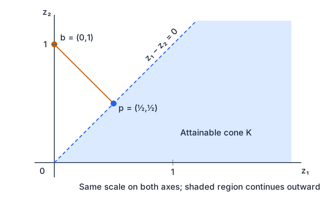
Why an outside point always has a certificate
The cone generated by finitely many columns is closed: it contains limits of its convergent sequences. This fact is needed for the nearest point to exist. For completeness, one way to see it is to reduce each nonnegative representation to a linearly independent subset of columns: a dependence lets us vary coefficients until one becomes zero without changing the represented vector. There are finitely many subsets; along a subsequence one independent subset stays fixed, and its coefficients converge to nonnegative limits. This is an original expansion of the finite-cone argument; see Bertsekas’ convex-analysis slides, “Farkas–Minkowski–Weyl Theorems,” part (a).
Suppose $b\notin K$. Let $p$ be its nearest point in $K$, measured with the Euclidean norm, and set $y=p-b\ne0$. For any $z\in K$, the segment $p+\tau(z-p)$, $0\le\tau\le1$, stays in $K$. Squared distance is smallest at $\tau=0$, so its right derivative is nonnegative:
\[\left.\frac{d}{d\tau}\|p+\tau(z-p)-b\|_2^2\right|_{\tau=0} =2(p-b)^T(z-p)\ge0.\]Thus $y^T(z-p)\ge0$. Both $0$ and $2p$ belong to the cone; substituting them gives $y^Tp\le0$ and $y^Tp\ge0$, hence $y^Tp=0$. Consequently,
\[y^Tz\ge0\quad(z\in K),\qquad y^Tb=y^T(p-y)=-\|y\|_2^2<0.\]Each column lies in $K$, so $A^Ty\ge0$. This proves the second alternative whenever the first fails. In the pictured example, $p=(1/2,1/2)^T$ gives $p-b=(1/2,-1/2)^T$; multiplying by two gives our simpler certificate. Any positive rescaling preserves a certificate.
From infeasibility to LP bounds
For a feasible system $Ax\le b$ with unrestricted $x$, nonnegative weights satisfying $A^Ty=c$ prove an upper bound on the linear objective:
\[c^Tx=y^TAx\le y^Tb.\]This explains the connection between contradiction certificates and dual bounds. It is the same weighted-constraint calculation with a different surviving coefficient vector. See MIT’s LP duality notes.
For an original derivation, suppose this feasible system also implies $c^Tx\le d$. Adding the strict opposite inequality $c^Tx>d$ is outside the non-strict form stated above. Instead apply the equality-form lemma to the columns of
\[B=\begin{bmatrix}A^T&0\\b^T&1\end{bmatrix},\qquad h=\begin{bmatrix}c\\d\end{bmatrix}.\]If there were no $y\ge0,s\ge0$ with $A^Ty=c$ and $b^Ty+s=d$, the lemma would give $(u,\alpha)$ such that
\[Au+\alpha b\ge0,\quad\alpha\ge0,\quad c^Tu+\alpha d<0.\]If $\alpha>0$, $x=-u/\alpha$ would satisfy $Ax\le b$ but $c^Tx>d$. If $\alpha=0$, take any feasible $x_0$; $x_0-tu$ stays feasible for $t\ge0$ and its objective grows without bound because $c^Tu<0$. Both contradict the assumed bound. Therefore the weights exist. Feasibility matters here: an empty system implies every inequality vacuously.
For a primal with $x\ge0$, the usual upper-bound dual condition becomes $A^Ty\ge c$, rather than equality. The Linear Programming page develops that primal–dual pair and optimality certificates. Farkas’ Lemma establishes the underlying alternative; a full strong-duality argument must also address optimal values and attainment.
Conditions and common mistakes
The following are supplementary invented counterexamples and deductions, not historical data.
- Keep the strict negative remainder. For $x\le1$ and $-x\le-1$, the weights $(1,1)$ yield $0\le0$. The system is feasible at $x=1$; replacing $b^Ty<0$ with $b^Ty\le0$ would falsely certify it.
- Do not allow negative weights on upper-bound inequalities. For $x\le1$ and $x\le2$, the weights $(1,-1)$ cancel $x$ and give $b^Ty=-1$. But both inequalities hold at $x=0$. Multiplying the second by $-1$ reverses its direction, so adding them as two upper bounds is invalid.
- A failed candidate is not a feasibility proof. For $x\le0$ and $-x\le-1$, $y=(1,0)$ fails to cancel the variable; $y=(1,1)$ works. The lemma guarantees existence, not that an arbitrary trial succeeds.
- Real feasibility differs from integer feasibility. $x=1/2$ is feasible over the reals and infeasible when $x$ must be an integer. The real-variable lemma cannot provide a certificate of the displayed kind for an integer-only obstruction.
- Check the full model and arithmetic. A displayed floating-point residual close to zero is not an exact cancellation. Compare numerical output against the original coefficients and signs. Exact fractions in this page let us check the certificates algebraically.
Practice: construct and interpret certificates
These are original exercises. Attempt each before opening its hint or solution.
1. Hand calculation: cancel two variables
For unrestricted $u,v$, show that $u+v\le1$, $-u\le-1$, and $-v\le-1$ cannot all hold. Give $A,b,y$, and check all certificate conditions.
Hint
Add all three rows with equal weights.
Worked solution
$A=\begin{bmatrix}1&1\-1&0\0&-1\end{bmatrix}$, $b=(1,-1,-1)^T$, and $y=(1,1,1)^T$. Then $y\ge0$, $A^Ty=(0,0)^T$, and $b^Ty=-1$. Adding the rows yields $0\le-1$.
2. Interpretation: when a certificate stops working
In the machine problem, what does the displayed certificate tell you at $q=80$? Does its nonnegative remainder prove feasibility? Supply separate evidence.
Hint
Distinguish a failed contradiction from an actual allocation.
Worked solution
The remainder is $260-3(80)=20$, so these weights give no contradiction. That fact alone does not prove feasibility. The allocation $(8/3,3,0)$ produces $260/3$ of each part, at least $80$, and respects the time bounds; it proves feasibility.
3. Logical reasoning: turn nonexistence into a solution
For $Ax=b$, $x\ge0$, suppose every $y$ satisfying $A^Ty\ge0$ also satisfies $b^Ty\ge0$. What follows? Why does this conclusion need the lemma’s existence assertion?
Hint
Which alternative has been excluded?
Worked solution
No infeasibility certificate exists, so there must be a nonnegative solution of $Ax=b$. Showing the alternatives cannot coexist would not suffice: that only rules out certificates when a solution is already known. The lemma also guarantees that one alternative always exists.
4. Application: an impossible ingredient blend
A hypothetical blend uses $u,v\ge0$ kilograms of two feeds. Ingredient supply is $2u+v$ units. Availability requires $u\le2$, $v\le1$, while demand requires $2u+v\ge6$. Give a certificate in upper-bound form, including the nonnegativity rows. What changes if demand is $5$?
Hint
Weight the two availability bounds to reproduce the ingredient coefficients.
Worked solution
Order the rows as $u\le2$, $v\le1$, $-2u-v\le-6$, $-u\le0$, $-v\le0$. The weights $y=(2,1,1,0,0)^T$ are nonnegative, cancel both variables, and yield $0\le4+1-6=-1$. With demand $5$ the remainder is zero; $(u,v)=(2,1)$ meets the demand exactly. A certificate can ignore some rows without ceasing to certify the full system.
References and further learning
- Julius Farkas, Theorie der einfachen Ungleichungen (1902), bibliographic record: verified title, author, volume, and pp. 1–27; publisher record and DOI. These records do not verify a historical numerical example, and the original full text was unavailable during preparation.
- L. V. Kantorovich, Mathematical Methods of Organizing and Planning Production, Example 1 and Table 1, pp. 369–370: the published machine rates and production question used here; the 90-set target and Farkas certificate are our modern calculations.
- Gabriele Farina, MIT Nonlinear Optimization, Lecture 6 (2025), §L6.2: an accessible explanation of inequality certificates and separation.
- Michel Goemans, MIT Advanced Algorithms, Lecture 3 (September 19, 2001), §§1–2: equality and inequality forms, projection proof, and the next steps toward LP duality. The archive adds a cover page; the lecture itself is dated 2001.
- Dimitri Bertsekas, Convex Analysis and Optimization lecture slides: consult “Farkas–Minkowski–Weyl Theorems” for finite-cone closedness and the geometric formulation.
- MIT 6.854, LP duality notes: move from impossibility certificates to objective bounds and strong duality.