Optimization
Linear programming
Derive linear models, improving exchanges, and optimality certificates from Kantorovich's machine allocation and Dantzig's assignment problem.
Kantorovich’s problem: maximize complete sets of parts
Linear programming (LP) chooses quantities or activity levels to optimize a linear objective while satisfying linear restrictions. Its production-planning origins make the distinction between an objective and a restriction concrete.
Kantorovich’s 1939 monograph grew from a Plywood Trust problem. Its opening example uses metalworking machines to explain the same allocation issue. Here are the rates from his Example 1 and Table 1; each finished item needs one of each part. He explicitly labels this example illustrative. See the original example, pp. 369–370 in the English translation.
| Machine group | Number of machines | Part I per machine-day | Part II per machine-day |
|---|---|---|---|
| Milling machines | 3 | 10 | 20 |
| Turret lathes | 3 | 20 | 30 |
| Automatic turret lathe | 1 | 30 | 80 |
The following algebra is a modern re-derivation using these published rates. We treat working time as divisible and retain exact fractional production rates. A daily rate need not be a whole number of items; a whole-item count requires a separate rounding or scheduling interpretation. The source’s Table 2, p. 371, lists whole-number totals of $77$ for the separately balanced plan and $86$ for the specialized plan. Our exact continuous calculations below give $77.82$ and $86.67$. We use Table 1’s rates rather than treating Table 2’s integer entries as exact fractional-time equations.
Derive the decision variables from working time
Let $m,t,a$ be machine-days devoted to Part I in the milling, turret, and automatic groups. One machine-day means one machine working for one day. Thus $m=2$ means two of the three available milling machine-days go to Part I. If every machine works for the full day, the remaining times for Part II are $3-m$, $3-t$, and $1-a$.
The three identical machines in a group can share an allocation in different ways; $m$ measures their total time, not a count of machines permanently assigned to a part. The model assumes constant rates, additive output, and no changeover time or setup cost. Time cannot be negative or exceed availability:
\[0\le m\le3,\qquad0\le t\le3,\qquad0\le a\le1.\]Multiply each allocated time by its production rate. The daily quantities of Parts I and II are
\[P=10m+20t+30a,\] \[Q=20(3-m)+30(3-t)+80(1-a).\]Producing all machines’ fastest parts gives Part II alone. That makes $230$ parts but no complete items. The relevant objective is complete sets, not the sum of unmatched parts.
Let $z$ be the common output of each part. Requiring $P=Q=z$ gives a linear program:
\[\begin{aligned} \text{maximize}\quad &z\\ \text{subject to}\quad &10m+20t+30a=z,\\ &20(3-m)+30(3-t)+80(1-a)=z,\\ &0\le m,t\le3,\quad0\le a\le1,\quad z\ge0. \end{aligned}\]The equalities encode the need for matching parts. The bounds encode available working time. The objective asks for the largest matching output. These full-use and equal-output constraints follow the source’s general Problem A, pp. 371–372. Full utilization and exact matching are the formulation used here; a model allowing idling or surplus parts would express those choices with different constraints.
A balanced plan can still waste productive capacity
One plausible rule is to make each machine group produce equal quantities of both parts. For milling machines, $10m=20(3-m)$ gives $m=2$. Similarly,
\[20t=30(3-t)\ \Longrightarrow\ t=\frac95,\] \[30a=80(1-a)\ \Longrightarrow\ a=\frac8{11}.\]This plan produces
\[z=20+36+\frac{240}{11} =\frac{856}{11}\approx77.82.\]A feasible plan satisfies every constraint; an optimal plan has the best objective among feasible plans. This plan is feasible: every group balances its own parts. But the plant needs balance only in the combined output. That leaves room to specialize groups and make more complete sets with the same machinery.
Eliminate the balance equation to see the tradeoff
Expanding $P=Q$ gives
\[30m+50t+110a=230.\]Solve for $m$ and substitute into $z=P$:
\[m=\frac{230-50t-110a}{30},\] \[z=\frac{230}{3}+\frac{10}{3}t-\frac{20}{3}a.\]The new objective tells us how a change in one group affects total output after the other group restores the part balance. Increasing turret time on Part I helps; increasing automatic time on Part I hurts. Their raw Part I rates, $20$ and $30$, did not reveal this tradeoff.
Because $t\le3$ and $a\ge0$, the rewritten objective is at most
\[z\le\frac{230}{3}+\frac{10}{3}(3)=\frac{260}{3}.\]Try $t=3$ and $a=0$. The balance equation then requires $m=8/3$, within its bounds. Check both outputs:
\[P=10\left(\frac83\right)+20(3)=\frac{260}{3},\] \[Q=20\left(3-\frac83\right)+80=\frac{260}{3}.\]The feasible plan reaches the bound, so its optimal daily rate is $260/3\approx86.67$ complete sets. All turret time goes to Part I, all automatic time to Part II, and milling supplies the remaining balance. We derived this answer from the actual historical example’s rates; we will now derive an exchange procedure and an independent optimality certificate for the same problem.
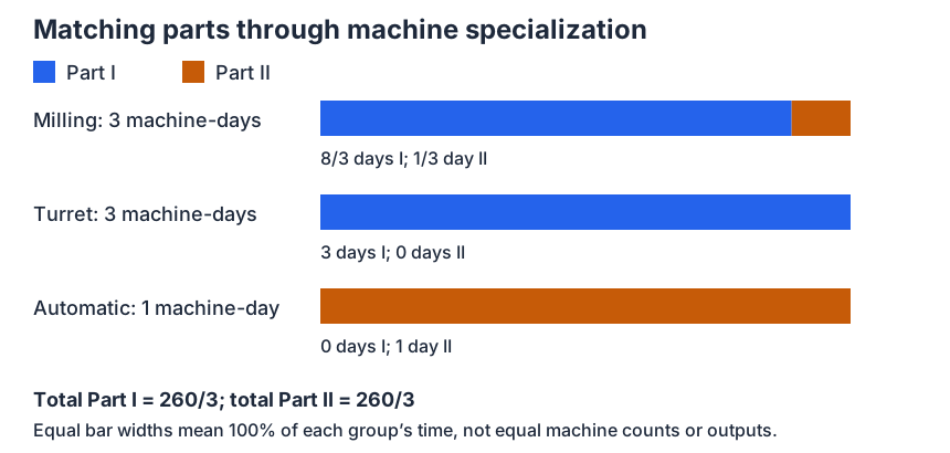
Definition and notation: generalizing the historical models
Working time, part balance, and later assignment activities fit the following general model.
A linear program optimizes a linear objective subject to linear equalities and inequalities. More precisely, affine expressions (linear expressions plus constants) are allowed. A general form is
\[\begin{aligned} \text{minimize}\quad &c^Tx+d\\ \text{subject to}\quad &Gx\le h,\\ &Ex=f. \end{aligned}\]Here $x\in\mathbb R^n$ contains the decision variables, the quantities we choose. The fixed vector $c$ gives their costs, and $c^Tx=\sum_{j=1}^n c_jx_j$ multiplies each quantity by its cost and adds. The constant $d$ changes the reported value but not which $x$ is best. In this general notation, $n$ counts variables, $m$ inequality rows, and $p$ equality rows; this $m$ is a dimension, not milling time. Matrices $G\in\mathbb R^{m\times n}$ and $E\in\mathbb R^{p\times n}$ store constraint coefficients; $h\in\mathbb R^m$ and $f\in\mathbb R^p$ store their limits. Inequalities are componentwise: every row must hold. Maximizing $c^Tx$ is equivalent to minimizing $-c^Tx$. See Boyd and Vandenberghe, §4.3.
A feasible point satisfies every constraint. The feasible region is the set of those points. An optimal solution is a feasible point with the best objective value; the point and its value are different objects. For matrix notation prerequisites, see the matrix-decomposition overview.
Historical data and problem statements are cited at their point of use. Unless explicitly attributed, the algebraic derivations and explanatory examples are our own.
Read the historical feasible region before walking along its edges
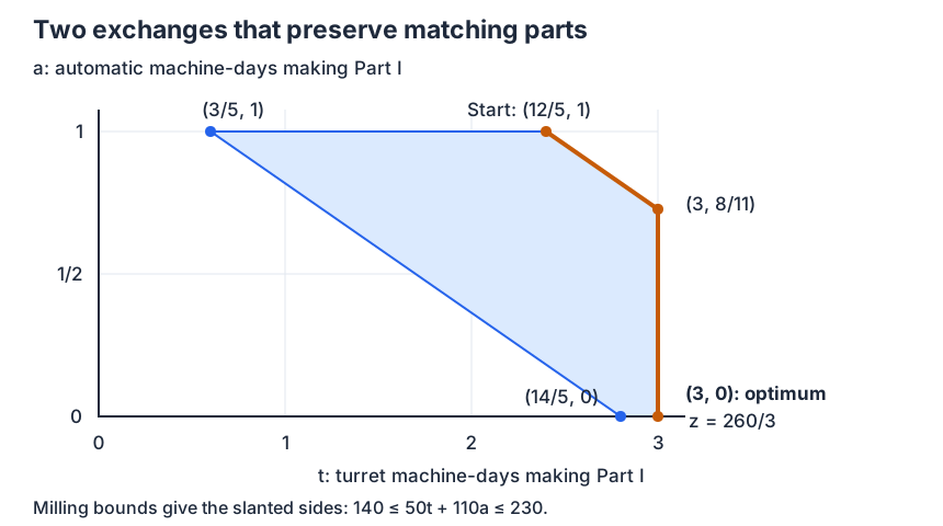
Eliminating $m$ leaves two coordinates, $t$ and $a$. Its lower and upper limits become
\[140\le50t+110a\le230,\qquad 0\le t\le3,\quad0\le a\le1.\]A linear inequality selects one side of a line, a half-plane. The intersection here is a polygon; in higher dimensions such an intersection is a polyhedron. A vertex, or corner, cannot be written as an average of two distinct feasible points. The region is convex: any line segment between feasible plans stays feasible because each linear constraint is preserved under weighted averages. Convexity works through mixtures of this same machine model and distinguishes convex feasible sets from convex objective functions.
Dantzig’s problem: a plan with too many alternatives to enumerate
Dantzig’s wartime work involved procurement, supply, deployment, and training. After the war he was asked to mechanize planning that had largely been done by hand. His oral history dates the LP model to June 1947 and simplex to August. See his firsthand account.
His later history illustrates the computational obstacle with 70 people assigned to 70 jobs, giving a benefit $v_{ij}$ when person $i$ fills job $j$. There are $70!>10^{100}$ possible complete assignments. See Dantzig (2002), p. 43. This is an example in his retrospective account, not a reproduced military dataset.
Derive one variable for each possible activity
Let $x_{ij}=1$ mean that person $i$ takes job $j$, and $x_{ij}=0$ mean otherwise. Each person gets one job, and each job gets one person:
\[\sum_{j=1}^{70}x_{ij}=1\quad(i=1,\ldots,70),\] \[\sum_{i=1}^{70}x_{ij}=1\quad(j=1,\ldots,70).\]There are $4900$ activity variables and $140$ stated balance equations, although one equation is redundant: summing either family gives the same total of $70$. The benefit of the plan is
\[\text{maximize}\quad\sum_{i=1}^{70}\sum_{j=1}^{70}v_{ij}x_{ij}.\]The literal assignment problem requires binary variables. Replacing that requirement by $x_{ij}\ge0$ gives an LP relaxation, a continuous model with the same balances and objective. For example, a two-person subproblem permits all four entries to be $1/2$. That point describes fractional allocations rather than a literal assignment. The distinction matters: integrality is an additional question, not part of the definition of an arbitrary LP.
Why this assignment relaxation can still return a whole assignment
For these particular one-person/one-job balances, every vertex of the LP region is a $0$–$1$ assignment. Consequently there is an integral optimum for any linear benefit objective, although tied optima can also include fractional points. See Goemans’s matching notes, Theorem 1.6.
Here is the mechanism. Draw a connection between person $i$ and job $j$ whenever $0<x_{ij}<1$. Every person or job with one such connection must have at least two: a single fractional entry cannot complete a row or column whose sum is the integer $1$. In this finite network, following connections eventually yields a cycle. It alternates between people and jobs, so its length is even. Add a sufficiently small $\epsilon$ to alternate cycle entries and subtract it from the others. Reversing the signs gives a second plan. Both preserve the row and column sums and nonnegativity, and their average is the original plan. Hence a fractional plan is not a vertex.
For the two-person illustration, the all-$1/2$ matrix is the average of the two whole assignments
\[\begin{bmatrix}1&0\\0&1\end{bmatrix},\qquad \begin{bmatrix}0&1\\1&0\end{bmatrix}.\]Linearity makes the fractional plan’s benefit their average, so at least one whole assignment is as good. This special structure explains how LP can solve Dantzig’s assignment model without enumerating $70!$ plans. It does not imply that every LP has integer vertices.
Compare this with the machine problem. There an activity variable measured working time; here it records a possible person–job pairing. The same row-and-column organization turns a complicated plan into linear balances. Enumerating every complete assignment is unnecessary if an algorithm can use this structure.
A military program meant a plan or schedule. Dantzig recalled Koopmans suggesting the name “linear programming” in 1948, and described replacing planning ground rules with an explicit objective. See Dantzig (2002), pp. 43 and 46. In the machine problem, we saw why that matters: “balance every group separately” makes a permissible plan but fails to maximize completed output.
Simplex: turn the historical machine problem into improving exchanges
Dantzig recalled initially rejecting a walk along feasible edges as inefficient. Examining matrix columns led him to a useful algorithm that he then recognized as equivalent to that edge walk. See Origins of the Simplex Method.
Here we demonstrate the modern simplex viewpoint on Kantorovich’s published machine rates. This is our re-derivation, not a claim that Kantorovich used Dantzig’s later algorithm. The balance equation and objective are
\[30m+50t+110a=230,\qquad z=10m+20t+30a.\]Start at a feasible corner
Set milling Part I time to its lower bound $m=0$ and automatic Part I time to its upper bound $a=1$. The remaining time follows from the balance:
\[t=\frac{230-110}{50}=\frac{12}{5},\qquad z=78.\]This is a corner of the balanced feasible region: two variable bounds fix the point once the balance is imposed. It produces $78$ of each part.
Exchange automatic time for turret time
Keep $m=0$, but let $a$ decrease. To preserve matching output,
\[t=\frac{23}{5}-\frac{11}{5}a,\qquad z=92-14a.\]A decrease of one unit in $a$ requires an increase of $11/5$ in $t$ and improves output by $14$. We cannot continue past the turret limit. Setting $t=3$ gives
\[a=\frac8{11},\qquad z=\frac{900}{11}\approx81.82.\]The limiting bound determines where the exchange must stop.
Exchange automatic time for milling time
Now keep $t=3$ and continue decreasing $a$. The equations become
\[m=\frac83-\frac{11}{3}a,\qquad z=\frac{260}{3}-\frac{20}{3}a.\]This time each unit decrease in $a$ improves output by $20/3$. At $a=0$, milling time is $8/3<3$, so automatic time reaches its lower bound first. We arrive at the optimum found above:
\[(m,t,a)=\left(\frac83,3,0\right),\qquad z=\frac{260}{3}.\]Both exchanges followed feasible edges and stopped when a bound became binding, meaning it held with equality. The objective coefficients changed because each exchange had to maintain the part balance. This is the role of reduced costs: measure improvement after compensating changes in the other active variables.
Generalize the exchange as a basis pivot
In equality standard form $Ax=b$, $x\ge0$, assume $A$ has $r$ independent rows, meaning no row is a linear combination of the others. A basis selects $r$ independent columns, making a square system with a unique solution. Set nonbasic variables to zero and solve $A_Bx_B=b$ for the basic variables. A nonnegative result is a basic feasible solution. A pivot exchanges one selected column for another; the feasibility limit determines the leaving variable. For example, introduce nonnegative remaining times $s_m,s_t,s_a$ for Part II:
\[m+s_m=3,\qquad t+s_t=3,\qquad a+s_a=1.\]A slack variable records the difference between an upper bound and the bounded quantity. Here the slacks are time not assigned to Part I; that time makes Part II, so it is not idle machine capacity. Together with $30m+50t+110a=230$, these equations put the historical problem in equality standard form. At our starting corner the basic variables can be $t,s_m,s_t,a$, with nonbasic $m=s_a=0$. The first exchange brings $s_a$ into the basis and drives $s_t$ to zero; the second brings $m$ in and drives $a$ to zero. See MIT’s basis and simplex notes.
A Phase I auxiliary LP minimizes artificial variables measuring constraint violations to find a feasible start. A zero minimum supplies a feasible solution; a positive minimum proves infeasibility. See Goemans, §2.5. A zero basic variable makes a basis degenerate; pivots may then leave the point unchanged. Suitable pivot rules prevent cycling. See MIT’s algorithm notes.
Certify that no feasible plan exists
Farkas’ Lemma explains how to prove infeasibility directly. For a system $Ax\le b$ with unrestricted variables (including any variable bounds as explicit rows), exactly one exists: a feasible point, or nonnegative row weights $y$ satisfying $A^Ty=0$ and $b^Ty<0$. Adding the weighted constraints would then require $0\le b^Ty<0$, a contradiction. See Farina, Theorem L6.1.
For the machine data above, a hypothetical requirement of at least $90$ of each part is impossible: weighting the two output requirements and selected time bounds gives $0\le260-3(90)=-10$. The separate Farkas’ Lemma page derives those weights, explains the geometric separation behind them, and connects infeasibility certificates to dual bounds.
Kantorovich’s resolving multipliers: prove the machine plan is optimal
Why should turret time go to Part I when the automatic lathe has the higher Part I rate? Kantorovich’s resolving multipliers compare weighted output across alternative uses of each machine. His Appendix I develops this method and its optimality argument. See §§1–3 of the appendix.
We can construct such weights directly from the mixed milling group. To find weights that certify the already-derived mixed allocation, require a milling machine to have the same weighted output under its two uses. Thus choose nonnegative part weights satisfying
\[10\lambda_1=20\lambda_2.\]Normalize their sum to one. This gives $\lambda_1=2/3$, $\lambda_2=1/3$. They value the two parts relative to each other, not at market prices.
| Group | Weighted Part I rate | Weighted Part II rate | Larger weighted output |
|---|---|---|---|
| Milling | $10(2/3)=20/3$ | $20(1/3)=20/3$ | Tie: may split time |
| Turret | $20(2/3)=40/3$ | $30(1/3)=10$ | Part I |
| Automatic | $30(2/3)=20$ | $80(1/3)=80/3$ | Part II |
The weights recover our allocation: specialize turret and automatic time, then split milling time to balance the parts. More importantly, they bound every balanced plan.
Because $P=Q=z$ and the weights sum to one,
\[z=\frac23P+\frac13Q.\]A day’s time on each machine cannot contribute more than the larger of its two weighted rates. With three milling, three turret, and one automatic machine-days,
\[z\le3\left(\frac{20}{3}\right) +3\left(\frac{40}{3}\right) +\frac{80}{3} =\frac{260}{3}.\]Our allocation attains this bound. Thus the multipliers give a certificate that no other allocation can produce more. Assigning time to a strictly smaller weighted rate would create a gap in the certificate; mixing is possible where the weighted rates tie. This is the mechanism behind the complementary-slackness conditions below.
Duality: from the historical certificate to a general bound
This section develops duality as an optimality certificate for our production models. For systematic sign rules, a strong-duality proof through Farkas’ lemma, and the extension to Lagrangians and KKT conditions, continue to Optimization duality.
Dantzig recalled meeting von Neumann on October 3, 1947, when von Neumann connected LP to game theory, the study of choices whose outcomes depend on other participants, and outlined duality. See Dantzig (2002), p. 44. The machine certificate gives us a concrete way to read that idea: one optimization chooses activities; another chooses weights that bound what any activities can achieve.
Write the dual of the historical model itself
Let $h_{j1},h_{j2}$ be the two allocated times in group $j$, with capacity $N_j$ and rates $r_{j1},r_{j2}$ from Table 1. Our full-use equations are $h_{j1}+h_{j2}=N_j$, and the two part totals equal $z$. Assign part weights $\lambda_1,\lambda_2$ summing to one and a capacity value $w_j$ for each group. To bound every time allocation, require
\[w_j\ge r_{j1}\lambda_1,\qquad w_j\ge r_{j2}\lambda_2.\]Then, using the full-use equations,
\[z=\sum_j\sum_{k=1}^2\lambda_k r_{jk}h_{jk} \le\sum_j w_jN_j.\]The corresponding dual minimizes that last bound:
\[\begin{aligned} \text{minimize}\quad&3w_M+3w_T+w_A\\ \text{subject to}\quad&\lambda_1+\lambda_2=1,\\ &w_M\ge10\lambda_1,\quad w_M\ge20\lambda_2,\\ &w_T\ge20\lambda_1,\quad w_T\ge30\lambda_2,\\ &w_A\ge30\lambda_1,\quad w_A\ge80\lambda_2. \end{aligned}\]Here $M,T,A$ index milling, turret, and automatic groups, and $\lambda_k$ weights the output balance for part $k$. These multipliers are unrestricted in sign because the primal has equality balances and full-use equations. We may treat $z$ as unrestricted: the output equalities and nonnegative times already imply $z\ge0$. Our positive choice $\lambda=(2/3,1/3)$ and $w=(20/3,40/3,80/3)$ is dual feasible and attains $260/3$. The part weights and machine-time values are related, but they measure different things.
Generalize to inequality resource limits
The primal is the original optimization problem; its dual searches for a best bound obtained from the constraints. Dual signs depend on how the primal is written. For resource upper limits, rather than the historical full-use equalities, a common production form and its dual are
\[\begin{array}{lll} \text{Primal:}&\max c^Tx&Ax\le b,\ x\ge0,\\ \text{Dual:}&\min b^Ty&A^Ty\ge c,\ y\ge0. \end{array}\]Here $A$ has one row per resource and one column per activity; $b$ gives capacities, $c$ gives profits, and $y$ contains one nonnegative price per resource. The dual requires the priced inputs for every product to cover its profit. Weak duality says every dual feasible value bounds every primal feasible value:
\[c^Tx\le (A^Ty)^Tx=y^TAx\le y^Tb.\]Nonnegativity of $x$ justifies the first inequality and nonnegativity of $y$ the last. Strong duality says that if the primal is feasible with a finite optimal value, both problems attain that value. See MIT’s duality notes. Dual signs depend on the primal form: for a maximization primal, an equality row has an unrestricted dual variable, and an unrestricted primal variable has an equality dual constraint. See Goemans, §4.2.
Complementary slackness
For feasible $x,y$ in the displayed primal–dual pair, optimality is equivalent to
\[y_i\bigl(b_i-(Ax)_i\bigr)=0\quad\text{for every resource }i,\] \[x_j\bigl((A^Ty)_j-c_j\bigr)=0\quad\text{for every product }j.\]These are the complementary slackness conditions; see Goemans, §4.3. In this production form, a resource with unused capacity must have zero optimal price; a produced product must have input value exactly equal to its profit. The converse implications need not hold: a binding resource can have price zero. For example, maximize $x_1$ with $0\le x_1,x_2\le1$. The optimal point $(1,1)$ binds both upper limits, but dual prices $(1,0)$ value the second limit at zero.
To see the conditions algebraically, split the duality gap, the difference between the upper bound and earned profit:
\[b^Ty-c^Tx=y^T(b-Ax)+x^T(A^Ty-c).\]Every summand is nonnegative. The gap is zero exactly when all the displayed products vanish.
What the historical multipliers say about extra machinery
The weighted rates also value available machine time. Around our optimum, an extra machine-day has the following potential contribution to matching output:
| Extra machine-day | Bound on added complete-set output |
|---|---|
| Milling | $20/3$ |
| Turret | $40/3$ |
| Automatic | $80/3$ |
When attained locally, these rates are shadow prices, changes in optimal output when capacity is relaxed. We can verify their meaning using the original machine equations.
Add $\delta$ automatic machine-days, keeping the three milling and three turret machine-days. If the same specialization remains optimal, turret makes Part I, automatic makes Part II, and milling satisfies
\[10m+60=20(3-m)+80(1+\delta).\]Solving gives
\[m=\frac83+\frac83\delta,\qquad z=\frac{260}{3}+\frac{80}{3}\delta.\]For $0\le\delta\le1/8$, $m\le3$, so this allocation is feasible. The same multipliers certify its bound, and the extra automatic time really adds $80\delta/3$ complete sets. Beyond $\delta=1/8$, the formula demands more milling time than exists. The plant must change which machine makes which part, so extrapolating the same shadow price is unjustified.
This turns the original production problem into a capacity decision: the useful value of a faster machine depends on whether the other machines can supply its matching parts.
Interactive example: replay the exchanges and change capacity
Explore Kantorovich’s published machine data
Published illustrative-data baseline: 3 milling, 3 turret, and 1 automatic machine-day, with the fixed Part I/II rates from Kantorovich, Example 1 and Table 1, p. 369. The allocations and exchanges are modern re-derivations using divisible time, full utilization, exact matching of parts, and no setup time. Fractional outputs are daily production rates. Capacity changes are hypothetical experiments.
The original-data baseline uses the counts and rates in Kantorovich’s Example 1 and Table 1, p. 369, taking one working day per machine. The lab preserves the full-use and equal-part-output constraints of Problem A, pp. 371–372. Its continuous re-derivation retains fractional rates; the source’s Table 2 reports whole-number outputs. Restore published baseline and replay resets all capacities to $(3,3,1)$ and returns to the start of our worked exchange sequence.
Start with Next worked exchange to follow the two exchanges above, from output $78$ through $900/11$ to $260/3$. The filled dot marks the current allocation; the orange ring marks the best attainable plan. Compare the Part I and Part II totals and the remaining possible gain.
Then change a capacity or select a scenario. The exchange sequence is the modern re-derivation above, not a reconstruction of a historical computation. The published rates stay fixed; changed capacities are hypothetical experiments, not historical observations. Capacity changes show the new optimal plan immediately. Try automatic capacity $1.125$ (the specialization threshold), then $2$: milling and turret time now make Part I exclusively, while automatic time splits between parts. Also try zero turret time or zero time for every group. The plot handles regions that collapse to a segment or point. Restore the published baseline to replay the exchanges. The capacity limits $0$–$10$ and minimum positive entry are interface choices, not historical machine limits.
Capacities are divisible machine-days between $0$ and $10$; positive entries must be at least $10^{-6}$ to keep the numerical comparisons reliable. Inputs, scenario selection, and buttons support keyboard use. Without JavaScript, the original allocation, two exchange calculations, static diagrams, and capacity-threshold derivation above provide the same starting points.
Two-variable lab: see the geometry and change the objective
The historical machine problem used three time variables and a matching equation. The following original workshop model gives a simpler two-coordinate plot for exploring the same linear structure. Its data are invented for this lab. The machine derivation above is the historical worked example; this lab supplies an accessible two-dimensional visualization.
Let $x_1$ and $x_2$ be divisible batches of products A and B. Assume every batch can be sold at the stated profit.
| Per batch | Product A | Product B | Available |
|---|---|---|---|
| Machine hours | 1 | 1 | 4 |
| Material units | 2 | 1 | 5 |
| Profit units | 3 | 2 | — |
Resource limits describe what we can do
Start with the quantities we control: batches $x_1$ and $x_2$. The table gives the restrictions
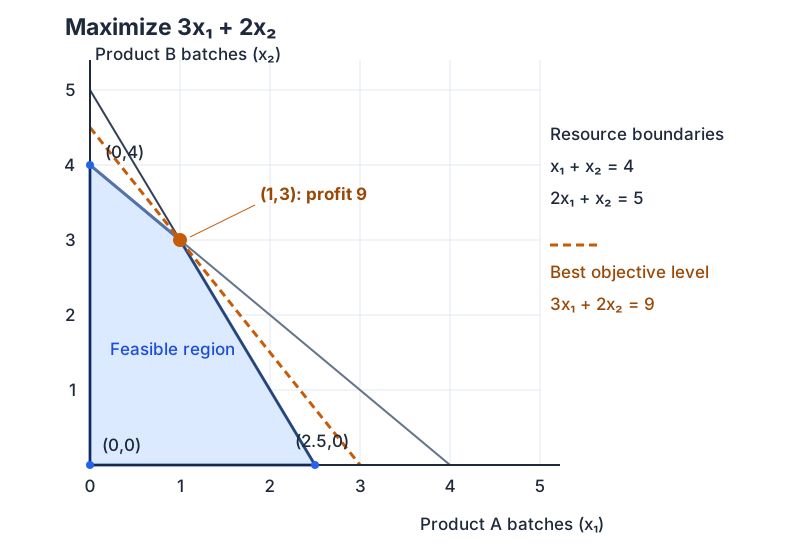
\[x_1+x_2\le4,\qquad2x_1+x_2\le5,\qquad x_1,x_2\ge0.\]For example, $(0,0)$, $(0,2)$, and $(1,3)$ all fit these limits. The constraints alone give us several possible plans, with no instruction about which one to choose.
Choose a profit objective
In our workshop, a ground rule such as “produce the higher-profit product first” is a choice of strategy. To evaluate that strategy, we need a stated goal: total profit. A batch of A earns $3$ profit units and a batch of B earns $2$, so our objective is $z=3x_1+2x_2$. Combining that objective with the restrictions gives
\[\begin{aligned} \text{maximize}\quad &z=3x_1+2x_2\\ \text{subject to}\quad &x_1+x_2\le4,\\ &2x_1+x_2\le5,\\ &x_1,x_2\ge0. \end{aligned}\]The first constraint measures hours, the second measures material, and nonnegativity excludes negative production. Check units within each row: the hour coefficients multiply batches to produce hours. Coefficients and capacities are assumed known and fixed during the plan.
This is $\max c^Tx$ subject to $Ax\le b$, $x\ge0$, with
\[A=\begin{bmatrix}1&1\\2&1\end{bmatrix},\qquad b=\begin{bmatrix}4\\5\end{bmatrix},\qquad c=\begin{bmatrix}3\\2\end{bmatrix}.\]Each row of $A$ records one resource restriction. Each column records the inputs for one activity: A consumes $(1,2)^T$, while B consumes $(1,1)^T$. This is the same row-and-column organization used in the historical machine exchanges.
Geometry of this supplementary model
An inequality such as $x_1+x_2\le4$ describes one side of a line, a half-plane. In more dimensions it is a half-space. Intersecting finitely many such sets and equality boundaries gives a polyhedron. It is convex: the entire line segment between any two feasible points remains feasible. For example, the midpoint of $(0,4)$ and $(1,3)$ is $(1/2,7/2)$, which satisfies both resource constraints.
A vertex, or extreme point, cannot be expressed as a nontrivial weighted average of two distinct feasible points. In this example vertices are the polygon’s corners. Every feasible point is a weighted average of these corners; the linear objective has the same weighted-average property. Therefore no point inside this polygon can beat all its corners.
More generally, for the form $Ax=b$, $x\ge0$, a feasible LP with a finite optimum has an optimal vertex. This needs care for unrestricted formulations: minimizing $x_1$ over the line $x_1=0$, $x_2\in\mathbb R$ has optimal points but no vertices. See MIT’s LP algorithm notes.
For a nonzero objective vector, level lines contain points with the same objective value. Here $3x_1+2x_2=k$ is $x_2=k/2-(3/2)x_1$. Slide this line toward larger $k$ until it last touches the region. It touches at $(1,3)$ when $k=9$. Changing profits rotates the level lines and can change which corner wins.
Find the feasible corners
The axes and the two resource boundary lines enclose a polygon. On the horizontal axis $x_2=0$, the tighter upper bound is $x_1\le5/2$. On the vertical axis $x_1=0$, it is $x_2\le4$. Where the two resource lines intersect,
\[x_1+x_2=4,\qquad2x_1+x_2=5 \quad\Longrightarrow\quad x_1=1,\quad x_2=3.\]Thus the four corners are $(0,0)$, $(5/2,0)$, $(1,3)$, and $(0,4)$.
Evaluate the corners and check the plan
| Corner | $3x_1+2x_2$ |
|---|---|
| $(0,0)$ | $0$ |
| $(5/2,0)$ | $15/2=7.5$ |
| $(1,3)$ | $9$ |
| $(0,4)$ | $8$ |
The best plan is $x^{\star}=(1,3)^T$, with $z^{\star}=9$. It uses $1+3=4$ hours and $2+3=5$ material units, exactly the capacities. Greedily making only the higher-profit product A gives $7.5$, so per-batch profit alone does not determine the best mix.
Supplementary interactive example: change invented profits
Supplementary invented-data lab: which mix wins?
Supplementary invented-data example: the workshop data and default profits (3, 2) are teaching choices, not historical observations. Changing profits creates further hypothetical teaching scenarios. Goemans’s LP modeling notes, §1.1 supports the modeling method, not these numerical data.
This lab supplements the historical-data lab above. Its workshop capacities and profits are invented; Goemans’s modeling notes, §1.1 support the formulation method, not these numbers. Restore teaching example (3, 2) restores the default invented profits. All edits remain hypothetical teaching scenarios.
The constraints stay fixed. Change the two profit coefficients using the labeled number inputs; arrow keys work too. Try $(c_1,c_2)=(3,2)$, $(1,1)$, $(2,1)$, and $(0,0)$. The latter three reveal an optimal edge, another optimal edge, and a constant objective. The display lists all optimal corners and explains when their connecting segment, or the entire region, is optimal. Negative profits and empty inputs are handled too. The static figure and corner table remain useful without JavaScript.
Possible outcomes and misconceptions
| Outcome | Example | Reason |
|---|---|---|
| Unique optimum | The production example | Only $(1,3)$ achieves $9$. |
| Multiple optima | Maximize $x_1+x_2$ with the same constraints | Every point from $(0,4)$ to $(1,3)$ achieves $4$. |
| Infeasible | Require $x_1\ge2$ and $x_1\le1$ | No point satisfies both. |
| Unbounded objective | Maximize $x_1$ subject only to $x_1\ge0$ | Profit can grow without limit. |
An unbounded region need not give an unbounded objective. Minimize $x_1$ subject to $x_1\ge0$: the region extends forever, but the minimum is $0$.
The optimum need not be unique or integral. Maximize $x_1$ subject to $2x_1\le5$ and $x_1\ge0$: the LP optimum is $2.5$. Requiring $x_1$ to be an integer changes the optimum to $2$ and makes this an integer program. Simply rounding a continuous solution is unreliable: rounding $2.5$ upward violates the constraint.
Linearity concerns the expressions, not the number of variables. $3x_1+2x_2$ is linear; $x_1x_2$ and $x_1^2$ are not. A squared-error objective leads to a quadratic problem; see quadratic forms.
Equivalent forms and slack variables
A slack variable measures unused capacity. Write the workshop inequalities as
\[x_1+x_2+s_1=4,\qquad2x_1+x_2+s_2=5,\qquad x_1,x_2,s_1,s_2\ge0.\]For the feasible plan $(0,2)$, the slacks are $s_1=2$ hours and $s_2=3$ material units. At $(1,3)$ both are zero; those constraints are binding, meaning equality holds.
One common standard form is $\min c^Tx$ subject to $Ax=b$, $x\ge0$. Conventions vary, so always state the form. A $\ge$ inequality becomes an equality by subtracting a nonnegative surplus variable. A variable allowed to have either sign can be replaced by $x_j=u_j-v_j$ with $u_j,v_j\ge0$. These transformations preserve the original decisions and objective through the stated substitutions. See Boyd and Vandenberghe, §4.3.
Verify the lab optimum with the same bounding idea
Let $y_1$ be the price per machine hour and $y_2$ the price per material unit, both nonnegative. To bound profit, require each product’s input value to cover its profit: $y_1+2y_2\ge3$ for A and $y_1+y_2\ge2$ for B. The full stock is worth $4y_1+5y_2$; we want the smallest bound we can justify. This price problem is called the dual LP; the production problem is the primal LP. For our workshop it is
\[\begin{aligned} \text{minimize}\quad &4y_1+5y_2\\ \text{subject to}\quad &y_1+2y_2\ge3,\\ &y_1+y_2\ge2,\\ &y_1,y_2\ge0. \end{aligned}\]Choose $y_1=y_2=1$. Product A’s inputs are valued at $1+2=3$ and B’s at $1+1=2$, meeting the dual constraints. The total capacity is valued at $4+5=9$. Equivalently, add the two resource inequalities:
\[(x_1+x_2)+(2x_1+x_2)\le4+5 \quad\Longrightarrow\quad3x_1+2x_2\le9.\]Our feasible plan earns $9$, and this bound proves that no plan earns more. This certificate is easier to verify than rerunning an optimization algorithm.
From simplex to interior methods and software
The modeling, pivot calculations, and price certificates we have worked through became parts of a general framework. Dantzig’s Linear Programming and Extensions appeared in 1963 as RAND report R-366-PR, bringing together formulations, simplex, duality, and applications including transportation and games. See RAND’s publication record and downloadable chapters.
Practical success raised a worst-case question: how fast can running time grow with the input? A polynomial-time guarantee bounds the work by a fixed polynomial in input size, including coefficient bits. Khachiyan obtained such a guarantee in 1979; Karmarkar’s 1984 paper gave a different interior approach. See Karmarkar’s introduction.
Karmarkar’s normalized problem: move the current point to the center
Karmarkar’s paper works with a transformed LP of the form
\[\text{minimize }c^Tx,\qquad Ax=0,\quad\sum_{i=1}^n x_i=1,\quad x\ge0.\]The nonnegative coordinates summing to one form a simplex, a higher-dimensional triangle; this geometric set is distinct from the simplex algorithm. Suppose $u$ is a feasible current point with every $u_i>0$. The paper’s projective change of coordinates is
\[y_i=\frac{x_i/u_i}{\sum_j x_j/u_j}.\]At $x=u$, every numerator is $1$, so $y_i=1/n$: the current point becomes the center. To check feasibility as well as recentering, take the supplementary test system
\[A=\begin{bmatrix}2&-3&0\end{bmatrix},\qquad c=(0,0,1)^T,\] \[u=(1/2,1/3,1/6)^T.\]These are invented demonstration coefficients, not a dataset from Karmarkar’s paper. Here $Au=2(1/2)-3(1/3)=0$, the coordinates sum to $1$, and the cost is $1/6$. Substitution maps $u$ to $(1/3,1/3,1/3)^T$.
Let $D$ be the diagonal matrix with entries $u_i$. The inverse is
\[x=\frac{Dy}{\sum_j u_jy_j}.\]Substitute into $Ax=0$. Since the denominator is positive, the transformed balance is still linear:
\[ADy=0.\]For the test system, $AD=(1,-1,0)$, so its center satisfies $y_1-y_2=0$. Inverting the center recovers $u$. The original test problem has minimum $0$ at $x=(3/5,2/5,0)^T$: its balance and normalization hold, and its nonnegative objective $x_3$ is zero. This verifies a feasible start, transformed balance, inverse, and target, without claiming to execute the full algorithm.
This is a concrete reason for the normalized equations (coordinates summing to one) and homogeneous balances (right-hand side zero): the recentering preserves a linear balance. The algorithm takes a controlled step inside a ball in the transformed feasible space and maps back. Its full analysis also needs a potential function measuring progress; recentering alone is not the complete solver. See Karmarkar (1984), §§1.1–1.5.
Some simplex rules take exponentially many pivots on worst-case examples. Polynomial-time LP algorithms exist, including ellipsoid and interior-point methods; for rational data, complexity counts the bits encoding the coefficients as well as dimensions. See MIT’s algorithm notes.
Solve the supplementary workshop plan with software
SciPy’s linprog minimizes, so negate the profits. Its HiGHS interface supports simplex and interior-point methods. Check solver status before reading a candidate solution. See the official linprog documentation.
from scipy.optimize import linprog

result = linprog(
    c=[-3, -2],
    A_ub=[[1, 1], [2, 1]],
    b_ub=[4, 5],
    bounds=[(0, None), (0, None)],
    method="highs",
)
if not result.success:
    raise RuntimeError(result.message)

print(result.x)      # [1. 3.]
print(-result.fun)   # 9.0
print(result.slack)  # [0. 0.]
Floating-point output should be checked against the original constraints with an appropriate tolerance and scale. A tiny residual is different from exact feasibility. If a model is infeasible, inspect conflicting requirements; if unbounded, inspect missing limits rather than adding an arbitrary cap.
Practice problems
Attempt each problem before opening its hint or solution. Exercises 1–2 use the published machine rates with new questions; the other exercises are original illustrations.
1. Hand calculation: check the first machine exchange
Use Kantorovich’s rates and the plan $m=0$, $t=12/5$, $a=1$. Decrease $a$ to $9/10$ while keeping $m=0$. Find the new $t$, check both part outputs, and calculate the gain.
Hint
Use $50t+110a=230$. Calculate $P$ and $Q$ separately as a check.
Worked solution
The balance gives $t=(230-99)/50=131/50=2.62$, below the upper limit $3$. Then
\[P=20(131/50)+30(9/10)=397/5=79.4,\] \[Q=60+30(3-131/50)+80(1-9/10)=79.4.\]The gain is $79.4-78=1.4$, agreeing with $14(1/10)$ from the reduced objective.
2. Interpretation: when does extra automatic time stop following its shadow price?
A planner proposes adding $1/4$ automatic machine-day to the historical plant. They predict a gain of $(80/3)(1/4)=20/3$ complete sets using the current shadow price. Can the same optimal specialization achieve that gain?
Hint
Check the milling time required by the capacity-change formula, and compare it with the available three machine-days.
Worked solution
The formula requires $m=8/3+(8/3)(1/4)=10/3>3$, so the specialization is infeasible. The original shadow price applies only up to $\delta=1/8$ for this increase. Beyond that point, some automatic time must switch to Part I. The proposed gain is a bound from the old certificate, not an achieved gain.
3. Logical reasoning: can an interior point win?
Let $x$ be strictly inside a full-dimensional feasible region, meaning a small ball around it is feasible. Can it maximize $c^Tx$ when $c\ne0$? What changes if $c=0$?
Hint
Consider moving a small distance in direction $c$.
Worked solution
For sufficiently small $\epsilon>0$, $x+\epsilon c$ remains feasible. Its objective is $c^Tx+\epsilon c^Tc$, strictly larger since $c^Tc=\sum_jc_j^2>0$. Thus such an interior point cannot maximize a nonconstant objective. If $c=0$, every feasible point is optimal. The full-dimensional assumption matters: a point inside a line segment relative to that line can be optimal when the objective is constant along the line.
4. Practical application: a minimum-cost blend
A blend needs at least $6$ units of an ingredient. Each kilogram of feed A provides $2$ units and costs $3$; each kilogram of feed B provides $1$ unit and costs $2$. At most $2$ kilograms of A are available. Formulate and solve an LP, assuming divisible quantities and no other requirements.
Hint
Use a lower-bound inequality for ingredient demand and an upper bound for A supply. A provides ingredient more cheaply per unit.
Worked solution
Let $a,b$ be kilograms of the feeds. Minimize $3a+2b$ subject to $2a+b\ge6$, $0\le a\le2$, and $b\ge0$. Positive costs make over-supplying ingredient unnecessary here. On $2a+b=6$, cost is $3a+2(6-2a)=12-a$, minimized at $a=2$, $b=2$, costing $10$. For a certificate valid even with over-supply,
\[3a+2b=2(2a+b)-a\ge12-2=10.\]References and further learning
- L. V. Kantorovich, Mathematical Methods of Organizing and Planning Production (1939; English translation, 1960), full text: the production-planning motivation and original numerical examples.
- George B. Dantzig, INFORMS oral history, interviewed by Irv Lustig: firsthand recollections of military planning and early computation.
- George B. Dantzig, Linear Programming (2002), Operations Research 50(1), 42–47: the origins of the terminology and the connection to von Neumann and duality. This is a retrospective account.
- George B. Dantzig, Origins of the Simplex Method: his account of the different geometric viewpoints behind simplex, in an archival collection.
- N. Karmarkar, A New Polynomial-Time Algorithm for Linear Programming (1984), Combinatorica 4, 373–395: the original paper on the interior approach and its complexity guarantee.
- Boyd and Vandenberghe, Convex Optimization, §4.3: general LP notation, standard-form conversions, and connections to convex optimization.
- Michel Goemans, Lecture notes on bipartite matching, Theorem 1.6: why assignment LPs have integral vertices and how that connects LP to matching algorithms.
- Michel Goemans, MIT 18.310 linear programming notes: modeling examples, basic feasible solutions, and the primal–dual rules in §§4.2–4.3.
- MIT 6.854, Lecture 10: polyhedra, bases, and the geometric foundation of simplex.
- MIT 6.854, algorithms for solving LPs: the algebra of simplex pivots, reduced costs, and complexity limits.
- MIT 6.854, LP duality: bounds, optimality certificates, and strong duality.
- SciPy
linprogdocumentation: solver input conventions, return status, slacks, and HiGHS options. - George B. Dantzig, Linear Programming and Extensions, RAND R-366-PR (1963): historical textbook with downloadable chapters on formulations, simplex, duality, and applications.