Linear Algebra
Quadratic form
Read xᵀAx as a scalar quadratic expression, understand its geometry, and connect its curvature to matrix factorizations and optimization.
Definition
A real quadratic form is a function $q:\mathbb R^n\to\mathbb R$ of the form
\[q(x)=x^TAx=\sum_{i=1}^n\sum_{j=1}^n a_{ij}x_ix_j,\]where $A\in\mathbb R^{n\times n}$ is fixed and $x\in\mathbb R^n$ is a column vector. It is a homogeneous quadratic expression: every term is a product of two coordinates, with no linear or constant term. See MIT’s notes, §5.2.
The dimensions explain why the result is a scalar:
\[\underbrace{x^T}_{1\times n}\, \underbrace{A}_{n\times n}\, \underbrace{x}_{n\times1} \quad\longrightarrow\quad 1\times1.\]Compute $Ax$ first, then take its dot product with $x$: $q(x)=x\cdot(Ax)$. The matrix maps a vector to another vector; the quadratic form assigns that vector a number. When $A=I$, this number is the ordinary squared length $x^Tx=\lVert x\rVert_2^2$. More general matrices describe directional penalties and interactions between coordinates.
The examples, derivations, and exercises below are original illustrations of these concepts.
Reading and constructing the matrix
For a symmetric two-by-two matrix,
\[A=\begin{bmatrix}a&b\\b&c\end{bmatrix},\qquad q(x)=ax_1^2+2bx_1x_2+cx_2^2.\]The cross term occurs twice in the matrix product: once from $a_{12}x_1x_2$ and once from $a_{21}x_2x_1$. Therefore, to represent $3x_1^2+4x_1x_2+2x_2^2$ with a symmetric matrix, put half the cross-term coefficient in each off-diagonal position:
\[A=\begin{bmatrix}3&2\\2&2\end{bmatrix}.\]For $x=(1,-1)^T$, compute it both ways:
\[Ax=\begin{bmatrix}1\\0\end{bmatrix},\qquad x^T(Ax)=1,\] \[3(1)^2+4(1)(-1)+2(-1)^2=1.\]For three variables, the same rule gives
\[2x_1^2+3x_2^2+x_3^2+6x_1x_2-4x_1x_3 =x^T\begin{bmatrix}2&3&-2\\3&3&0\\-2&0&1\end{bmatrix}x.\]An absent interaction means a zero off-diagonal entry; it does not require the corresponding diagonal entry to vanish.
Why only the symmetric part matters
Any real square matrix can be split into symmetric and skew-symmetric parts:
\[S=\frac{A+A^T}{2},\qquad K=\frac{A-A^T}{2},\qquad A=S+K.\]Because $K^T=-K$ and a scalar equals its transpose,
\[x^TKx=(x^TKx)^T=x^TK^Tx=-x^TKx.\]Thus $x^TKx=0$ and
\[\boxed{x^TAx=x^TSx.}\]This proves why restricting to symmetric representatives loses no quadratic forms; see MIT’s Exercise 84 and Theorem 86. A quadratic form has a unique symmetric representative in a fixed basis, although adding any skew-symmetric matrix leaves the form unchanged.
For example,
\[A=\begin{bmatrix}2&5\\-1&3\end{bmatrix},\qquad S=\begin{bmatrix}2&2\\2&3\end{bmatrix}\]both produce $2x_1^2+4x_1x_2+3x_2^2$. To study the signs or geometry of this form, use the eigenvalues of $S$. Positive eigenvalues of a nonsymmetric $A$ alone do not suffice: \(A=\begin{bmatrix}1&4\\0&1\end{bmatrix}\) has only eigenvalue $1$, but $q(1,-1)=-2$.
Geometry: direction, scale, and level curves
For any real scalar $t$,
\[q(tx)=t^2q(x),\qquad q(-x)=q(x).\]Doubling a displacement multiplies its value by four. Reversing its direction leaves the value unchanged. The form is therefore generally not linear: it scales quadratically, and coordinate interactions prevent additivity.
For symmetric $A$, use the spectral theorem to write $A=Q\Lambda Q^T$, where the columns of the orthogonal matrix $Q$ are unit eigenvectors and $\Lambda$ contains eigenvalues. Setting $y=Q^Tx$ gives
\[q(x)=y^T\Lambda y=\sum_i\lambda_i y_i^2.\]The eigenvector coordinates remove cross terms. See MIT’s diagonalization argument. Since $Q$ preserves lengths, each $\lambda_i$ measures the penalty along a unit principal direction; the curvature of $q$ along that direction is $2\lambda_i$.
For a concrete rotation, let \(A=\begin{bmatrix}2&1\\1&2\end{bmatrix}\). Its unit eigenvectors are $(1,1)^T/\sqrt2$ and $(1,-1)^T/\sqrt2$, with eigenvalues $3$ and $1$. Hence
\[y_1=\frac{x_1+x_2}{\sqrt2},\qquad y_2=\frac{x_1-x_2}{\sqrt2},\qquad q(x)=3y_1^2+y_2^2.\]The level curve $q(x)=1$ is an ellipse with semiaxes $1/\sqrt3$ and $1$ along those two directions. A larger positive eigenvalue makes the same-value contour narrower in that direction.
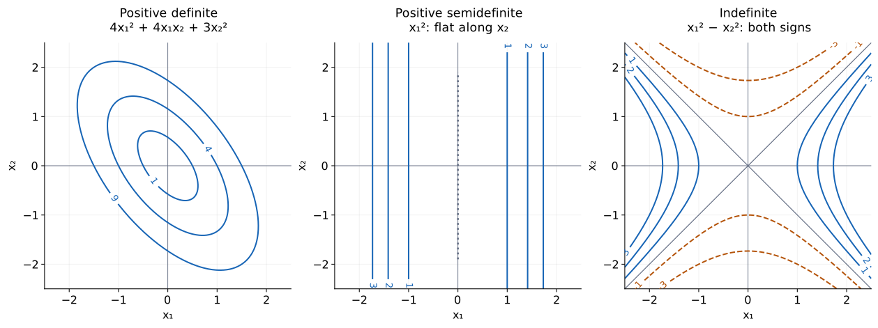
Read the figure as a map in the input plane, rather than a graph of height against position. The corresponding height function is a bowl, a trough, or a saddle.
Definiteness: what signs are possible?
Use the symmetric representative $S$ if the original $A$ is nonsymmetric.
| Type | Condition | Eigenvalues of $S$ | Example |
|---|---|---|---|
| Positive definite | $q(x)>0$ for all $x\ne0$ | All positive | $x_1^2+2x_2^2$ |
| Positive semidefinite | $q(x)\ge0$ for all $x$ | All nonnegative | $x_1^2$ |
| Negative definite | $q(x)<0$ for all $x\ne0$ | All negative | $-x_1^2-2x_2^2$ |
| Negative semidefinite | $q(x)\le0$ for all $x$ | All nonpositive | $-x_1^2$ |
| Indefinite | Takes both positive and negative values | Both signs occur | $x_1^2-x_2^2$ |
These sign tests follow from the diagonal sum above; compare MIT’s Theorem 86. Definite forms are also semidefinite under the non-strict definitions; “semidefinite but not definite” specifically allows a nonzero zero-value direction. The zero form is both positive and negative semidefinite.
Positive diagonal entries do not prove positivity in every direction. For \(A=\begin{bmatrix}1&2\\2&1\end{bmatrix}\), both coordinate axes give positive values, but $q(1,-1)=-2$. Conversely, negative off-diagonal entries need not prevent positive definiteness:
\[2x_1^2-2x_1x_2+2x_2^2=(x_1-x_2)^2+x_1^2+x_2^2.\]A zero value at a nonzero vector need not mean a flat direction. For the indefinite form $x_1^2-x_2^2$, $q(1,1)=0$ even though $A(1,1)^T\ne0$. For a positive semidefinite symmetric matrix, however, $q(x)=0$ forces all positive-eigenvalue coordinates to vanish, so $Ax=0$.
Completing the square and Cholesky
For $a>0$, direct expansion verifies
\[ax_1^2+2bx_1x_2+cx_2^2 =a\left(x_1+\frac ba x_2\right)^2+ \left(c-\frac{b^2}{a}\right)x_2^2.\]For \(A=\begin{bmatrix}4&2\\2&3\end{bmatrix}\), this becomes
\[q(x)=(2x_1+x_2)^2+(\sqrt2x_2)^2.\]This sum is strictly positive unless $x=0$. The transformation is $L^Tx$, with
\[L=\begin{bmatrix}2&0\\1&\sqrt2\end{bmatrix},\qquad A=LL^T,\qquad q(x)=\lVert L^Tx\rVert_2^2.\]Cholesky decomposition constructs such triangular sums of squares for symmetric positive-definite matrices. Its existence for SPD matrices is described by Higham. The remaining coefficient $c-b^2/a$ is the scalar Schur complement; for fixed $x_2$, it determines the minimum after allowing $x_1$ to adjust. Gallier, §2, develops the block version.
An orthogonal eigenvector transformation preserves lengths and reveals principal directions. The triangular Cholesky transformation instead rescales and mixes coordinates to make the penalty an ordinary squared length. These are two useful matrix decompositions with different purposes.
Derivatives and optimization
Expand $q(x+h)$ to see the first-order change:
\[q(x+h)-q(x)=h^TAx+x^TAh+h^TAh =h^T(A+A^T)x+h^TAh.\]The term quadratic in $h$ has no first-order contribution, so
\[\nabla q(x)=(A+A^T)x,\qquad \nabla^2q(x)=A+A^T.\]For symmetric $A$, these reduce to $2Ax$ and $2A$. The common factor $1/2$ in an objective cancels that $2$:
\[f(x)=\frac12x^TAx-r^Tx+d,\qquad \nabla f(x)=Ax-r,\qquad \nabla^2f(x)=A.\]$f$ is a quadratic function; its quadratic part is the form. If $A$ is SPD, its stationary point $x_\star$ solves $Ax_\star=r$. Substituting this equation and expanding gives
\[f(x)-f(x_\star)=\frac12(x-x_\star)^TA(x-x_\star)>0 \quad(x\ne x_\star),\]which proves it is the unique global minimum. A stationary point of an indefinite quadratic need not minimize it.
Least squares provides a practical example:
\[\lVert Bx-b\rVert_2^2=x^TB^TBx-2b^TBx+b^Tb.\]Its quadratic form is $x^TB^TBx=\lVert Bx\rVert_2^2$, so it is nonnegative. Independent columns of $B$ make it positive definite; otherwise some parameter changes cost nothing. See Higham’s Gram-matrix argument and the LU page’s normal-equation derivation.
Interactive example: change the coupling
The existing energy explorer below uses \(A=\begin{bmatrix}a&b\\b&c\end{bmatrix}\) and reports $q(x)$ for your chosen vector. Keep $a=4$, $c=3$, and $x=(1,-1)^T$: predict $q(x)=7-2b$ before moving the coupling slider. Then compare the flat and indefinite presets and their displayed zero or negative directions.
Explore a quadratic form and its directions
The colors show signs and relative magnitudes on a fixed input range. A zero value at your selected vector alone does not classify the entire form. Without JavaScript, use the completed-square example above: $b=2$ gives positive definiteness, $b=\sqrt{12}$ gives a flat direction, and $b=4$ gives an indefinite form. These boundaries concern all directions, even while $q(1,-1)$ may remain positive.
Practice problems
These four original exercises cover hand calculation, interpretation, logical reasoning, and application. Attempt each before revealing the hint or solution.
1. Hand calculation: build and evaluate
Find the symmetric matrix for $q(x)=5x_1^2-6x_1x_2+2x_2^2$ and evaluate $q(1,2)$ by both matrix multiplication and polynomial substitution.
Reveal a hint
Split the coefficient −6 equally between the two off-diagonal entries.
Reveal the worked solution
\(A=\begin{bmatrix}5&-3\\-3&2\end{bmatrix}\) and $Ax=(-1,1)^T$ at $x=(1,2)^T$. Thus $x^TAx=-1+2=1$. Substitution also gives $5-12+8=1$.
2. Interpretation: distinguish zero value from a flat direction
Compare $q_1(x)=(x_1+x_2)^2$ and $q_2(x)=x_1^2-x_2^2$. Both vanish at $v=(1,-1)^T$. Which is positive semidefinite? Which is indefinite? Does either satisfy $Av=0$?
Reveal a hint
Try the coordinate axes, then multiply each representing matrix by v.
Reveal the worked solution
\(A_1=\begin{bmatrix}1&1\\1&1\end{bmatrix}\) is PSD because $q_1$ is a square, and $A_1v=0$: adding any multiple of $v$ leaves $q_1$ unchanged. $A_2=\operatorname{diag}(1,-1)$ is indefinite because the two axes give opposite signs. Here $A_2v=(1,1)^T\ne0$; the zero value comes from cancellation, not a nullspace direction.
3. Logic: recover a symmetric matrix from its form
Suppose symmetric matrices $S,T$ satisfy $x^TSx=x^TTx$ for every $x$. Prove $S=T$. Why does the conclusion fail without symmetry?
Reveal a hint
Set D = S − T. Test coordinate vectors eᵢ and their sums eᵢ + eⱼ.
Reveal the worked solution
$e_i^TDe_i=d_{ii}=0$. For $i\ne j$,
\[(e_i+e_j)^TD(e_i+e_j)=d_{ii}+2d_{ij}+d_{jj}=0.\]Thus $d_{ij}=0$. Every entry of $D$ vanishes. Without symmetry, any nonzero skew-symmetric $K$ satisfies $x^TKx=0$ for all $x$, giving the same form as the zero matrix.
4. Application: minimize a coupled penalty
For \(A=\begin{bmatrix}4&2\\2&3\end{bmatrix}\) and $r=(6,5)^T$, minimize $f(x)=\frac12x^TAx-r^Tx$. Find the minimizer and prove it is global.
Reveal a hint
Solve Ax = r, then use the completed-square expression for the quadratic form to justify minimality.
Reveal the worked solution
$4x_1+2x_2=6$ and $2x_1+3x_2=5$ give $x_\star=(1,1)^T$, with $f(x_\star)=11/2-11=-11/2$. Writing $h=x-x_\star$ yields
\[f(x)-f(x_\star)=\frac12\left((2h_1+h_2)^2+2h_2^2\right).\]It is positive for every nonzero $h$, so the minimizer is unique and global.
Further learning
- MIT 14.102, §5.2: Quadratic Forms: follow the transition from polynomial expressions to eigenvalue sign tests. The displayed negative-semidefinite inequality in Theorem 86 is $\lambda_i\le0$; its accompanying prose contains a sign typo.
- Higham: What Is a Symmetric Positive Definite Matrix?: connect positive quadratic values with Gram matrices and Cholesky factors.
- Gallier: The Schur Complement and Symmetric Positive Semidefinite (and Definite) Matrices: extend scalar square completion to coupled blocks of variables.
Related pages
- Symmetric positive definite matrix
- Cholesky decomposition
- Schur complement
- Matrix factorization and decomposition
- LU decomposition
References
- Barczi, N. (2004). 14.102: Math for Economists, Lecture Notes, September 23. MIT, §5.2, Quadratic Forms.
- Higham, N. J. (2020). What Is a Symmetric Positive Definite Matrix?.
- Gallier, J. (2019). The Schur Complement and Symmetric Positive Semidefinite (and Definite) Matrices. University of Pennsylvania.