Linear Algebra
Matrix factorization and decomposition
Represent matrices as products of structured factors, and choose between LU, Cholesky, QR, and other decompositions.
Definition
A matrix factorization, also called a matrix decomposition, expresses a matrix as a product of matrices with useful structure. For example,
\[A = BC\]where $A \in \mathbb{R}^{m\times n}$, $B \in \mathbb{R}^{m\times r}$, and $C \in \mathbb{R}^{r\times n}$. The intermediate dimension $r$ makes the product compatible. A decomposition may have more than two factors.
The structure of the factors is what makes the representation useful. Triangular factors simplify linear solves; orthogonal factors preserve Euclidean lengths; diagonal factors expose independent scalings. Numerical linear algebra uses these structures to solve systems, least-squares problems, and eigenvalue problems. LAPACK’s guide to linear equations and orthogonal factorizations describe these uses.
Without additional conditions, a product representation need not be unique. For any invertible $S \in \mathbb{R}^{r\times r}$,
\[BC = (BS)(S^{-1}C).\]Conditions such as a unit diagonal or positive diagonal entries remove some of this freedom.
Intuition: one operation becomes a sequence
A matrix tells us how to transform a vector. Its columns are the images of the coordinate basis vectors: if $A$ has columns $a_1$ and $a_2$, then $Ax=x_1a_1+x_2a_2$. A factorization $A=BC$ describes the same transformation in stages:
\[x\ \xrightarrow{\ C\ }\ y=Cx\ \xrightarrow{\ B\ }\ BCx=Ax.\]The rightmost factor acts first. The factors are not pieces to add together; they are operations to compose. For example, let
\[C=\begin{bmatrix}2&0\\0&1\end{bmatrix},\qquad B=\begin{bmatrix}1&1\\0&1\end{bmatrix}.\]$C$ stretches the horizontal coordinate, while $B$ shears horizontally. For $x=(0,1)^T$, stretching and then shearing gives $BCx=(1,1)^T$. Reversing the order gives $CBx=(2,1)^T$. The operations have the same ingredients but different results.
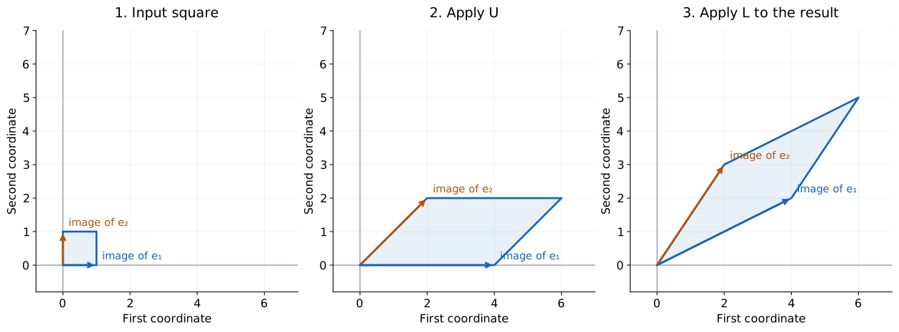
The factors can be simpler to work with even though their product is a dense matrix. A diagonal matrix scales coordinates independently. An orthogonal matrix rotates or reflects without changing lengths. A triangular matrix mixes coordinates in a one-way dependency pattern, making its equations solvable in sequence. See LAPACK’s discussion of orthogonal factors.
Why zeros in a factor matter
Compare the lower triangular system
\[\begin{bmatrix}2&0&0\\1&3&0\\4&-1&2\end{bmatrix} \begin{bmatrix}y_1\\y_2\\y_3\end{bmatrix} =\begin{bmatrix}2\\7\\6\end{bmatrix}.\]The first row determines $y_1=1$. Substituting it into the second gives $y_2=2$. With those two known, the third gives $y_3=2$. There is no need to solve all three unknowns simultaneously. The zero entries encode the dependency order: $y_1\to y_2\to y_3$. Upper triangular systems reverse that order.
Factorization does not make the original problem disappear. It performs the coupled work once, then stores a representation whose later uses are simpler.
Common decompositions
The table uses real matrices. A square matrix $Q$ is orthogonal when $Q^TQ=I$. In complex arithmetic, the corresponding notion is unitary, and the conjugate transpose $Q^*$ replaces $Q^T$.
| Decomposition | Form | Conditions and factor structure | Typical use |
|---|---|---|---|
| LU | $PA=LU$ | For general nonsingular square matrices; $P$ permutes rows, $L$ is unit lower triangular, and $U$ is upper triangular | Linear systems |
| Cholesky | $A=LL^T$ | Symmetric positive-definite $A$; $L$ is lower triangular with positive diagonal | Linear systems with positive-definite coefficients |
| QR | $A=QR$ | For $m\ge n$, the reduced form has $Q\in\mathbb{R}^{m\times n}$ with $Q^TQ=I$ and upper triangular $R\in\mathbb{R}^{n\times n}$ | Least squares with full column rank |
| Singular value decomposition (SVD) | $A=U\Sigma V^T$ | Any $m\times n$ matrix; full $U$ and $V$ are orthogonal, and $\Sigma$ is rectangular diagonal with nonnegative entries | Singular values and rank analysis |
| Symmetric eigendecomposition | $A=Q\Lambda Q^T$ | Real symmetric $A$; $Q$ is orthogonal, and $\Lambda$ is real diagonal | Eigenvalues and eigenvectors |
For the factor structures, see LAPACK’s LU routine, Cholesky routine, and Users’ Guide sections on QR, SVD, and symmetric eigendecomposition. LAPACK writes pivoted LU as $A=PLU$; its permutation matrix is the inverse of the one in $PA=LU$.
Why factor before solving?
Suppose $A$ is nonsingular and we want to solve
\[Ax=b.\]With pivoted LU, this becomes $LUx=Pb$. Introduce $y=Ux$, then solve
\[Ly=Pb,\qquad Ux=y.\]Forward substitution solves the lower triangular system, and backward substitution solves the upper triangular system. If another right-hand side arrives, the factors can be reused. LAPACK separates factorization and solve routines for this reason.
Worked example
Consider
\[A=\begin{bmatrix}4&2\\2&3\end{bmatrix}.\]It has both an LU decomposition and a Cholesky decomposition:
\[A= \begin{bmatrix}1&0\\\tfrac12&1\end{bmatrix} \begin{bmatrix}4&2\\0&2\end{bmatrix} = \begin{bmatrix}2&0\\1&\sqrt2\end{bmatrix} \begin{bmatrix}2&1\\0&\sqrt2\end{bmatrix}.\]Multiplying either pair recovers $A$. The LU factor has unit diagonal in its lower factor. The Cholesky upper factor is the transpose of its lower factor. These are different structured representations of the same matrix.
What the different decompositions reveal
LU exposes an elimination procedure
Elimination removes an unknown from later equations. $U$ stores the simplified equations; $L$ stores the multipliers needed to reconstruct the original ones. The same matrix can therefore be read as either an original coupled system or a record of how to solve it. The LU page works through that record explicitly.
Cholesky exposes a sum of squares
For SPD $A=LL^T$,
\[x^TAx=\lVert L^Tx\rVert_2^2.\]The quadratic expression on the left may mix coordinates. The right side writes it as ordinary squared length after a triangular change of coordinates. For the example \(A=\begin{pmatrix}4&2\\2&3\end{pmatrix}\),
\[4x_1^2+4x_1x_2+3x_2^2=(2x_1+x_2)^2+(\sqrt2x_2)^2.\]This is completing the square in matrix form. The Cholesky page explains why the positivity condition makes it possible.
QR separates direction from coordinate mixing
Columns of $Q$ form perpendicular unit directions. Columns of $R$ say how to combine those directions to recover the columns of $A$. For instance,
\[\begin{bmatrix}1&1\\1&-1\end{bmatrix} =\frac1{\sqrt2}\begin{bmatrix}1&1\\1&-1\end{bmatrix} \begin{bmatrix}\sqrt2&0\\0&\sqrt2\end{bmatrix}.\]The columns already point in perpendicular directions; $Q$ normalizes them, and $R$ restores their lengths. For columns that are not perpendicular, the off-diagonal entries of $R$ also record components along earlier directions. See LAPACK’s QR definition.
As a small least-squares example, fit one constant $x$ to measurements $(1,2,6)^T$. The design matrix is $B=(1,1,1)^T$. Reduced QR gives $q=B/\sqrt3$ and $r=\sqrt3$, so $rx=q^Tb$ gives $x=3$. The residual $b-Bx=(-2,-1,3)^T$ is perpendicular to $q$: its entries sum to zero. The fit captures the component in the model’s direction and leaves the perpendicular component as residual.
SVD finds input and output directions for stretching
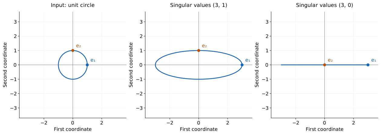
In $A=U\Sigma V^T$, $V^T$ expresses the input in perpendicular directions, $\Sigma$ scales those coordinates, and $U$ places them in output directions. For a square matrix, the orthogonal stages may rotate or reflect; the nonnegative diagonal entries of $\Sigma$ give the stretch factors. The relation $Av_i=\sigma_i u_i$ makes this interpretation precise. See LAPACK’s SVD definition.
For $A=\operatorname{diag}(3,1)$, a unit circle becomes an ellipse with semiaxes $3$ and $1$. If the second diagonal entry is instead zero, the circle collapses onto a line segment: an entire input direction is lost. This illustrates why zero singular values indicate rank loss. Small singular values mean that corresponding input changes produce small output changes, which become strongly amplified when a solve tries to reverse them.
Symmetric eigendecomposition finds directions that keep their orientation
An eigenvector is a nonzero vector whose image is a scalar multiple of itself. For
\[A=\begin{bmatrix}3&1\\1&3\end{bmatrix},\qquad A\begin{bmatrix}1\\1\end{bmatrix}=4\begin{bmatrix}1\\1\end{bmatrix},\qquad A\begin{bmatrix}1\\-1\end{bmatrix}=2\begin{bmatrix}1\\-1\end{bmatrix}.\]The two diagonal directions are stretched by $4$ and $2$. Normalize them to form $Q$, and the matrix becomes $Q\operatorname{diag}(4,2)Q^T$. The same directions are used for input and output. That differs from SVD, whose input and output directions can be different, even for square matrices. Symmetric matrices have an orthogonal eigenbasis; see LAPACK’s symmetric eigendecomposition. Negative eigenvalues reverse a direction, while singular values remain nonnegative.
Choosing a decomposition
For a general nonsingular square system, use pivoted LU. If the coefficient matrix is symmetric positive definite, Cholesky exploits that structure. For an overdetermined system with full column rank, QR solves the least-squares problem. If rank is uncertain, column-pivoted QR or SVD can help identify an effective numerical rank. See LAPACK’s linear-system factorizations and rank-sensitive least-squares discussion.
Interactive example: change the order
Before moving a slider, predict where the vector and the corners of the unit square will go. The experiment uses $C=\operatorname{diag}(s,1)$ and \(B=\begin{pmatrix}1&k\\0&1\end{pmatrix}\). Start with $s=2$, $k=1$, then reverse the order. Explain the difference using the intermediate vector, rather than only comparing final numbers.
Compose a scale and a shear
Practice problems
Try each problem before opening its hint or solution. The first two build hand-calculation fluency, the next two ask you to interpret or choose an approach, the next two develop logical reasoning, and the final two connect the concept to practical work. These are original exercises; the references support the mathematical concepts they use.
1. Hand calculation: compose two factors
Let
\[B=\begin{bmatrix}1&1\\0&1\end{bmatrix},\quad C=\begin{bmatrix}2&0\\0&3\end{bmatrix},\quad x=\begin{bmatrix}1\\2\end{bmatrix}.\]Compute $Cx$, $BCx$, and $CBx$. Are the last two vectors equal?
Reveal a hint
Apply the rightmost matrix first. Compare the two intermediate vectors.
Reveal the worked solution
$Cx=(2,6)^T$, so $BCx=(8,6)^T$. Conversely, $Bx=(3,2)^T$, so $CBx=(6,6)^T$. Scaling and shearing do not commute in this example.
2. Hand calculation: verify a factorization
Verify
\[\begin{bmatrix}2&1\\0&3\end{bmatrix} =\begin{bmatrix}1&1\\0&1\end{bmatrix}\begin{bmatrix}2&-2\\0&3\end{bmatrix}.\]Then apply the product to $(1,1)^T$, using the factors rather than the original matrix.
Reveal a hint
Check all four product entries, then track the intermediate vector.
Reveal the worked solution
The product entries are $2$, $-2+3=1$, $0$, and $3$. The right factor sends $(1,1)^T$ to $(0,3)^T$; the left factor sends that to $(3,3)^T$. Direct multiplication by the original matrix gives the same answer.
3. Thinking: select the structure you need
Choose a useful starting decomposition for each task, and explain your choice: (a) solve a nonsingular SPD system; (b) fit three parameters to 100 observations with a full-column-rank design matrix; (c) identify a direction that a matrix nearly destroys.
Reveal a hint
Ask whether you need a triangular solve, perpendicular model directions, or stretch factors.
Reveal the worked solution
(a) Cholesky exploits the SPD structure. (b) QR supplies an orthonormal model basis and a triangular least-squares solve without forming normal equations. (c) SVD identifies directions with small singular values. These choices follow the task and assumptions; several decompositions may exist for the same matrix.
4. Thinking: a small stretch can cause a large inverse response
Let $A=\operatorname{diag}(5,0.01)$. An output perturbation of size $0.001$ affects either the first or second coordinate. What change in the corresponding input coordinate is needed to account for it?
Reveal a hint
Reverse each stretch by dividing by its scale factor.
Reveal the worked solution
The first coordinate changes by $0.001/5=0.0002$. The second changes by $0.001/0.01=0.1$, which is 500 times larger. A weakly transmitted direction is difficult to recover accurately from perturbed output.
5. Logic: why the intermediate dimension bounds rank
Suppose $A=BC$ with $B\in\mathbb R^{m\times r}$ and $C\in\mathbb R^{r\times n}$. Prove $\operatorname{rank}(A)\le r$. What does this imply if $A$ has rank greater than $r$?
Reveal a hint
Every column of the product is a linear combination of columns of B.
Reveal the worked solution
For every vector $x$, $Ax=B(Cx)$ lies in the column space of $B$. Thus $\operatorname{Col}(A)\subseteq\operatorname{Col}(B)$ and $\operatorname{rank}(A)\le\operatorname{rank}(B)\le r$. An exact factorization through only $r$ intermediate coordinates is impossible when $\operatorname{rank}(A)>r$.
6. Logic: why factors need normalization
If $A=BC$ and $\alpha\ne0$, show that $A=(\alpha B)(\alpha^{-1}C)$. Does this prove every structured decomposition is nonunique?
Reveal a hint
Distinguish an unrestricted product from a product whose factors have extra conditions.
Reveal the worked solution
Scalar cancellation gives the same product. It proves nonuniqueness for unrestricted nonzero factors. It does not preserve every normalization: multiplying a unit lower triangular factor by $\alpha\ne1$ destroys its unit diagonal, for example. Uniqueness theorems concern factors satisfying all the stated conditions.
7. Applied: combine repeated measurements
A sensor reports $2$, $3$, and $7$ for one constant quantity. With equal observation weights, use reduced QR for $B=(1,1,1)^T$ to find the least-squares estimate. What are the residuals?
Reveal a hint
Use $q=B/\sqrt3$, $r=\sqrt3$, and solve $rx=q^Tb$.
Reveal the worked solution
$q^Tb=12/\sqrt3$, so $x=4$. The residuals are $(-2,-1,3)^T$. Their sum is zero, so the residual is perpendicular to the model column. Equal weighting makes this estimate the arithmetic mean; different weights would change the objective.
8. Applied: undo a graphics transformation
A graphics pipeline first scales horizontal coordinates by $2$, then applies horizontal shear $k=1/2$. A point $(1,2)^T$ is transformed. Find its output and the order of operations needed to recover the input.
Reveal a hint
A forward sequence is undone in reverse order.
Reveal the worked solution
Scaling gives $(2,2)^T$; shearing gives $(3,2)^T$. To undo the pipeline, first subtract half the vertical coordinate from the horizontal coordinate, giving $(2,2)^T$, then divide the horizontal coordinate by $2$. Algebraically, $(BC)^{-1}=C^{-1}B^{-1}$, whose rightmost factor undoes $B$ first.
Further learning
- LAPACK: orthogonal factorizations: connect length-preserving transformations to least squares.
- LAPACK: QR and SVD: compare the factor dimensions and the different directions they reveal.
- LU and Cholesky: continue with elimination records, positive energy, and their dedicated practice sets.
Related pages
References
- Anderson, E., et al. (1999). LAPACK Users’ Guide, third edition. SIAM. Linear Equations.
- Anderson, E., et al. (1999). LAPACK Users’ Guide. Orthogonal Factorizations and Linear Least Squares Problems and QR Factorization.
- Anderson, E., et al. (1999). LAPACK Users’ Guide. QR Factorization with Column Pivoting.
- Anderson, E., et al. (1999). LAPACK Users’ Guide. Singular Value Decomposition.
- Anderson, E., et al. (1999). LAPACK Users’ Guide. Error Bounds for the Symmetric Eigenproblem, opening definition of the eigendecomposition.
- LAPACK (2011). DGETRF and DPOTRF, version 3.3.1. Routine documentation for LU and Cholesky factors.