Cholesky decomposition

Definition

For a real symmetric positive-definite (SPD) matrix $A\in\mathbb{R}^{n\times n}$, the Cholesky decomposition, or Cholesky factorization, is

where $L$ is lower triangular with strictly positive diagonal entries. This factor exists and is unique. Equivalently, $A=R^TR$ with $R=L^T$ upper triangular. SPD means

See van de Geijn’s definition and existence theorem. For complex Hermitian positive-definite matrices, the form is $A=LL^{\ast}$, where $L^{\ast}$ is the conjugate transpose. LAPACK’s ZPOTRF documentation gives the complex convention.

This is a structured matrix decomposition. Unlike the unit lower triangular factor in LU decomposition, the Cholesky factor generally has diagonal entries other than $1$.

Intuition: positive energy becomes ordinary squared length

A quadratic form is the scalar $q(x)=x^TAx$. Think of it as an energy or penalty assigned to a displacement $x$. For the real symmetric matrix \(A=\begin{pmatrix}4&2\\2&3\end{pmatrix}\),

The cross term couples the coordinates. Completing the square gives

Cholesky finds the triangular coordinate transformation that makes this mixed quadratic expression a sum of squares. If $L$ is invertible, a nonzero $x$ cannot become the zero vector under $L^T$, so the squared length is strictly positive. That explains the SPD condition. See Higham’s discussion of positive-definite quadratic forms.

Positive definite does not mean that every entry of the matrix is positive. For example, \(\begin{pmatrix}2&-1\\-1&2\end{pmatrix}\) gives

Conversely, \(\begin{pmatrix}1&2\\2&1\end{pmatrix}\) has positive entries but gives $x^TAx=-2$ for $x=(1,-1)^T$. The condition concerns every direction, not the signs of individual entries.

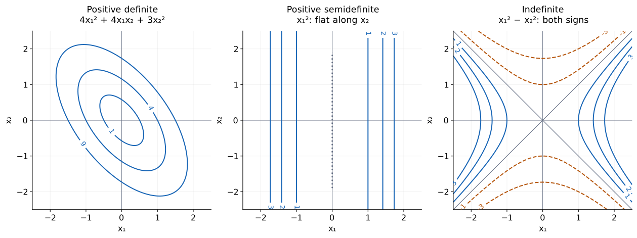
The semidefinite example has a direction that costs no energy. The indefinite example has a direction with negative energy, so it cannot equal a squared Euclidean length for all $x$. These geometric differences correspond to zero or invalid square-root pivots in the usual algorithm.

The factor is a table of dot products

Write the rows of $L$ as $r_1,\ldots,r_n$. Then $a_{ij}=r_i\cdot r_j$. In the two-variable example,

Their squared lengths are $4$ and $3$, and their dot product is $2$. These are precisely the two diagonal entries and the off-diagonal entry of $A$. Triangularity lets us construct these vectors one coordinate at a time: give the first row its length, match the next row’s dot product with it, then choose the remaining coordinate to supply the remaining squared length. This is the Gram-matrix interpretation of $LL^T$; see the FLAME definition and algorithm.

A triangular square root has a specific meaning

$A=LL^T$ resembles $a=\sqrt a\sqrt a$, but generally $L^2\ne A$. The transpose matters. In our example, the upper-right entry of $L^2$ is zero, while $a_{12}=2$. A symmetric matrix square root satisfying $S^2=A$ is a different factorization. Cholesky chooses a triangular factor because it supports sequential computation and solves.

Deriving the algorithm

Equating entries in $A=LL^T$ gives

Compute columns in order, for $j=1,\ldots,n$:

then, for $i=j+1,\ldots,n$,

Empty sums are zero. Entries above the diagonal remain zero. These recurrences are the lower triangular counterpart of the elementwise Cholesky algorithm presented by Higham.

Each diagonal entry supplies what is still missing

For a two-by-two matrix, write

Matching $LL^T$ to $A$ yields three requirements:

First choose $\ell_{11}=\sqrt a$. Next choose $\ell_{21}=b/\sqrt a$ to match the shared component. Finally choose $\ell_{22}=\sqrt{c-b^2/a}$ to supply the squared length that the first coordinate has not supplied.

For $a=4$, $b=2$, $c=3$, the second row needs total squared length $3$. Its first coordinate is $1$, already contributing $1$. The remaining coordinate must contribute $2$, so it is $\sqrt2$. This makes the subtraction inside the recurrence concrete: subtract the contribution already accounted for, then take the square root of what remains.

The same remainder appears when completing the square:

For $a>0$, a positive remainder means the second direction still has positive energy. A zero remainder leaves a flat direction. A negative remainder gives a negative-energy direction. In higher dimensions, the Schur complement is the matrix version of this remainder.

Why the square roots are positive

Partition an SPD matrix as

Here $\alpha>0$. For nonzero $z$, set $x=(-c^Tz/\alpha,z)^T$. Then

Thus the Schur complement $B-cc^T/\alpha$ is SPD. Inductively factor it as $KK^T$, and obtain

The positive square root and each successive column are uniquely determined. This gives an inductive existence and uniqueness proof; see the FLAME notes for a full treatment.

Worked example

Let

It is SPD because, for $x\ne0$,

The recurrences give

Therefore

To solve $Ax=b$ for $b=(6,5)^T$, first solve $Ly=b$:

Then solve $L^Tx=y$ to obtain $x_2=1$ and $x_1=1$. Direct substitution confirms $A(1,1)^T=b$.

A second example: shared and independent variation

Let $z_1,z_2$ be independent random variables with mean zero and variance one, and set

Then $\operatorname{Var}(u_1)=4$, $\operatorname{Var}(u_2)=1+2=3$, and $\operatorname{Cov}(u_1,u_2)=2$. Both outputs share $z_1$, which produces covariance. The independent $z_2$ supplies the remaining variance of the second output. In matrix notation, $u=Lz$ and $\operatorname{Cov}(u)=LL^T=A$. See Stata’s covariance-transformation explanation.

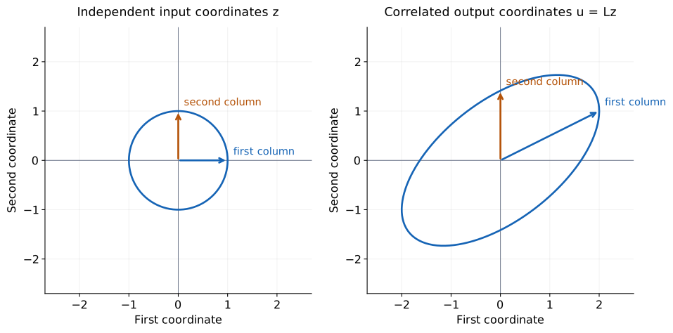
Reading the same factor in different ways gives different intuitions: $L^T$ removes the coupling from a quadratic energy, while $L$ introduces a desired covariance into independent inputs. The algebraic identity is the same, but the direction of the transformation and the problem being solved differ.

What a nearly zero remainder tells us

For

positive $\varepsilon$ gives an SPD matrix. At $\varepsilon=0$, the two rows represent the same underlying direction and the matrix is singular. For small positive $\varepsilon$, the second independent contribution is tiny: the system is close to losing a direction. A triangular solve divides by $\sqrt\varepsilon$, explaining why small changes can matter greatly. This example illustrates the distinction between existence and numerical sensitivity discussed below.

Applications and computational cost

For an SPD linear system, solve $Ly=b$ by forward substitution, then $L^Tx=y$ by backward substitution. Reuse $L$ for additional right-hand sides. LAPACK’s DPOTRS routine implements this factor-and-solve workflow.

The determinant follows from the product:

See Higham’s determinant identity; the logarithmic formula follows by taking logs of positive diagonal entries.

Conventional dense Cholesky costs $\frac13 n^3+O(n^2)$ floating-point operations, counting multiplication and addition separately, and two triangular solves cost $O(n^2)$ per right-hand side. The cubic leading term is half that of conventional dense LU. Only one triangular factor needs storage. See the cost discussion in the FLAME notes.

Numerical behavior and limitations

For SPD input, standard Cholesky needs no pivoting and has small backward error: the computed factor $\widehat L$ satisfies $A+\Delta A=\widehat L\widehat L^T$ for a small perturbation $\Delta A$. An ill-conditioned system can still have a large solution error. In floating-point arithmetic, a nearly singular SPD matrix may cause a nonpositive computed pivot. Higham discusses stability and breakdown.

Symmetry alone is insufficient. An indefinite matrix does not have the positive-diagonal Cholesky factor defined above. Positive-semidefinite matrices can have triangular square-root factors with zero diagonal entries, but uniqueness and the standard algorithm’s divisions no longer follow. See Higham’s semidefinite discussion. For symmetric indefinite systems, LAPACK uses pivoted factorizations with block diagonal $D$ instead.

History

The original problem was adjusting a measured network

André-Louis Cholesky was a French artillery officer working in the army’s geographic service. When the French triangulation network was being revised, officers needed ways to adjust the measured network with greater speed, convenience, and precision. Benoît’s account of Cholesky’s work identifies this practical problem as the setting for his least-squares calculation procedure. See Benoît’s account, translated by Richard W. Cottle.

What does adjusting a network mean? Consider a simplified surveying example in a flat plane. Three measured triangle angles might add up to $180^\circ+\varepsilon$, although the geometric condition requires $180^\circ$. Corrections $v_1,v_2,v_3$ must satisfy

There are infinitely many possible corrections. If the observations have equal weight, minimizing $v_1^2+v_2^2+v_3^2$ gives $v_1=v_2=v_3=-\varepsilon/3$. A network has many conditions sharing the same observations, so the corrections must be calculated together. This example illustrates the adjustment problem; an actual geodetic model also accounts for the Earth’s curvature and the geometry of the network.

The original question was therefore: how can we calculate small corrections that make a whole measured network consistent, with a procedure people can carry out reliably? Least squares specifies the desired corrections. Cholesky’s contribution concerns the numerical work needed to obtain them.

Why this produced normal equations

The title of Benoît’s 1924 paper refers to fewer equations than unknowns. This describes the condition equations for observation corrections, rather than the overdetermined regression problem commonly used to introduce least squares today. De Falguerolles, §5.2, explains this formulation.

In modern notation, let $v\in\mathbb R^m$ contain corrections and let $C\in\mathbb R^{p\times m}$ contain $p<m$ independent linearized conditions. For equal observation weights, solve

Introduce Lagrange multipliers $\lambda\in\mathbb R^p$:

Stationarity and the constraints give

Thus an underdetermined correction problem becomes a square system for the multipliers. Its coefficient matrix $N=CC^T$ is symmetric. Full row rank makes it positive definite, since

For positive observation weights collected in a diagonal matrix $W$, minimizing $\frac12v^TWv$ instead gives $N=CW^{-1}C^T$ and $v=W^{-1}C^T\lambda$. This follows from the same stationarity calculation.

In regression, the familiar route is instead

Both routes produce a Gram matrix, positive definite under the appropriate rank assumption. The historical distinction is what the unknowns represent: observation corrections and their multipliers in network adjustment, or fitted parameters in regression. See de Falguerolles, §§5.1–5.2.

The 1910 method organized the solve into two stages

Cholesky’s surviving manuscript is dated 2 December 1910, establishing that the method existed by then. The exact invention date is unknown. See Brezinski (2005), p. 217.

The following uses modern notation for the construction described in Brezinski (2006), pp. 283–286. Instead of solving $N\lambda=d$ directly, find a lower triangular $L$ such that

Introduce an intermediate vector $y=L^T\lambda$. The calculation becomes

The first equation gives $y_1$, then $y_2$, and so on. The second gives $\lambda_p$, then $\lambda_{p-1}$, and so on. Matching entries of $N$ and $LL^T$ supplies the square-root recurrences given earlier in this article. The factorization organizes a coupled system into successive scalar calculations.

Cholesky also described the calculation layout, use of a Dactyle mechanical calculator, and checks for mistakes. These details mattered because the work was performed by people, including soldiers with limited mathematical training. His discussion already included finite-precision errors; concern for numerical reliability was present before electronic computers. See Brezinski (2006), pp. 285–286.

Publication in 1924 and wider adoption after 1944

Cholesky died in 1918. Commandant Benoît published the method in 1924, six years later. The publication date differs from the manuscript date. See Cottle’s translation and publication note.

Henry Jensen’s 1944 comparison of methods for normal equations reached John Todd, who used it in his 1946 course at King’s College London. Leslie Fox brought the method to the National Physical Laboratory. Work by Fox, Huskey, Wilkinson, and Turing in 1948 developed its numerical analysis, followed by dissemination through textbooks. See Brezinski (2005), pp. 216–217. This connects with the postwar accuracy questions discussed in the LU history.

The scope broadened and the accuracy question became more precise

Cholesky’s manuscript already considers general square systems. Its construction, written in modern notation for nonsingular $B$, is

Solve the symmetric system for $\lambda$, then recover $x$. See Cholesky’s manuscript, systems I–III, pp. 221–223.

Modern numerical analysis distinguishes algebraic equivalence from computational accuracy. For nonsingular square $B$,

Forming normal equations can therefore make the computation much more sensitive to rounding. A stable Cholesky solve of the resulting matrix does not undo this effect. QR or SVD can avoid forming the Gram matrix when that loss of accuracy matters. See ALAFF, §4.2.5 and LAPACK’s least-squares methods.

The accuracy question also became more explicit: can a computed solution be interpreted as the exact solution of a nearby problem, and how does conditioning turn that perturbation into solution error? LAPACK’s backward-error discussion expresses these as separate quantities. This refines the original aim of reliable calculation rather than replacing it.

Electronic computing added another implementation problem: moving data through memory efficiently. LAPACK reorganizes algorithms into blocks so that much of the work uses matrix-matrix operations. The identity $A=LL^T$ remains the same, while the arrangement of the computation changes with the machine.

The factor became useful beyond solving equations

A modern Cholesky factor can also represent a covariance structure. Suppose $\Sigma=LL^T$ is a positive-definite covariance matrix and $z$ has independent standard normal components. Then

Here the factor generates correlated observations rather than solving for unknowns. Stata’s explanation of multivariate-normal simulation gives this construction. It demonstrates how the same triangular factor acquired additional uses without changing its mathematical definition.

The historical thread is thus a continuing problem of usable computation: first, obtain least-squares corrections for measured networks; then, establish precise accuracy guarantees and efficient implementations; and, in additional applications, use the factor itself as a representation of a positive-definite matrix.

Interactive example: vary the remaining energy

The experiment uses symmetric \(A=\begin{pmatrix}a&b\\b&c\end{pmatrix}\). Predict the sign of $c-b^2/a$ before changing the shared coefficient $b$. When the factorization fails, find a direction with zero or negative energy. A failure here is a consequence of the chosen matrix, rather than a reason to take the square root of a negative number. The calculations follow the Cholesky recurrences in the FLAME notes.

Practice problems

Try each problem before opening its hint or solution. The first two build hand-calculation fluency, the next two ask you to interpret or choose an approach, the next two develop logical reasoning, and the final two connect the concept to practical work. These are original exercises; the references support the mathematical concepts they use.

1. Hand calculation: factor and solve

Find $L$ with positive diagonal, solve $Ax=b$, and compute $\det A$ for

2. Hand calculation: construct three rows

Compute the Cholesky factor and determinant of

3. Thinking: diagnose the failed square root

Compare \(A_1=\begin{pmatrix}1&2\\2&5\end{pmatrix}\) and \(A_2=\begin{pmatrix}1&2\\2&3\end{pmatrix}\). Which admits positive-diagonal Cholesky? For the other, exhibit a negative-energy direction.

4. Thinking: interpret correlation near one

For the covariance matrix \(A_\rho=\begin{pmatrix}1&\rho\\\rho&1\end{pmatrix}\) with $0\le\rho<1$, find $L$. Interpret its second diagonal when $\rho=0.9$ and as $\rho\to1$.

5. Logic: prove positivity and examine uniqueness

If $L$ is an invertible real lower triangular matrix, prove $LL^T$ is SPD. Why does the uniqueness theorem require a positive diagonal?

6. Logic: identify the factor of a leading block

If $A=LL^T$ is an SPD Cholesky factorization, show that the upper-left $k\times k$ block of $L$ is the Cholesky factor of the upper-left $k\times k$ block of $A$.

7. Applied: generate correlated sensor errors

Two sensors need zero-mean errors with covariance \(\Sigma=\begin{pmatrix}4&1\\1&1\end{pmatrix}\). Construct the errors from independent zero-mean, unit-variance variables $z_1,z_2$. Verify the two variances, covariance, and correlation.

8. Applied: minimize a quadratic penalty

An optimization step minimizes

Derive the system for its minimizer and solve it with Cholesky. Why is the stationary point the unique minimum?

Further learning

• FLAME: Notes on Cholesky Factorization: study the full proof, algorithm, operation count, and accompanying exercises.
• Higham: What Is a Symmetric Positive Definite Matrix?: connect energy, eigenvalues, and positivity conditions.
• ALAFF: why normal equations can lose accuracy: understand why a stable factorization is only one part of a reliable least-squares computation.
• Stata: multivariate-normal simulation: connect exercise 7 to a complete covariance-generation example.

Related pages

• Symmetric positive definite matrix

• Matrix factorization and decomposition
• LU decomposition

References

1. van de Geijn, R. A. (2011). Notes on Cholesky Factorization. University of Texas at Austin. Definition, proof, algorithm, and operation count.
2. Higham, N. J. (2020, August 11). What Is a Cholesky Factorization?. Determinant identity, numerical stability, and semidefinite extensions.
3. Anderson, E., et al. (1999). LAPACK Users’ Guide, third edition. SIAM. Linear Equations. Real and complex factorizations and triangular solves.
4. LAPACK (2011). ZPOTRF and DPOTRS, version 3.3.1. Complex Cholesky factorization and solves using an existing factor.
5. Cholesky, A.-L. (1910, December 2). Sur la résolution numérique des systèmes d’équations linéaires. Manuscript reproduced in Brezinski (2005), §4, pp. 221–229.
6. Benoît, Commandant (1924). Note sur une méthode de résolution des équations normales provenant de l’application de la méthode des moindres carrés à un système d’équations linéaires en nombre inférieur à celui des inconnues (Procédé du Commandant Cholesky). Bulletin géodésique, 2, 67–77. DOI. Publication history described in Brezinski (2005).
7. Benoît, Commandant. Account of Cholesky’s life and geodetic work, translated by R. W. Cottle in 1975 and circulated in NA Digest, February 18, 1990.
8. Brezinski, C. (2005). La méthode de Cholesky. Revue d’histoire des mathématiques, 11(2), 205–238. Full text. Historical investigation and reproduction of the original manuscript.
9. Brezinski, C. (2006). The life and work of André Cholesky. Numerical Algorithms, 43, 279–288. Author-uploaded full text.
10. de Falguerolles, A. (2019). Cholesky and the Cholesky decomposition: a commemoration by an applied statistician. Journal de la Société Française de Statistique, 160(2), 83–96. Sections 5.1–5.2 distinguish fitting and compensation.
11. van de Geijn, R. A., and Myers, M. Advanced Linear Algebra: Foundations to Frontiers. §4.2.5, Why using the Method of Normal Equations could be bad.
12. Anderson, E., et al. (1999). LAPACK Users’ Guide. Linear Least Squares Problems and Further Details: Error Bounds for Linear Equation Solving. See also the LAPACK project description for blocked computation.

13. StataCorp. Stata 6: Simulating multivariate normal observations. Cholesky factors as covariance transformations.

14. Higham, N. J. (2020, July 21). What Is a Symmetric Positive Definite Matrix?. Quadratic-form interpretation and positivity conditions.