Optimization
Simplex method
Derive basis exchanges, reduced costs, and the ratio test from a historical production problem, then certify the answer and find a feasible start.
A production plan needs a rule for its next improvement
The simplex method solves a linear program by exchanging variables in a basis: a small set of independent columns that determines a candidate solution. Primal simplex keeps the plan feasible while seeking a better objective. A pivot usually moves along an edge to another corner; a degenerate pivot can change the basis without moving the point. We will derive these operations before stating the general algorithm. See Goemans, §§2–3.
Start with the production difficulty behind linear programming: maximizing total parts can leave unmatched components. Kantorovich’s 1939 monograph gives the following published illustrative data, not factory measurements. Every finished item needs one of each part. See Example 1 and Table 1, printed pp. 369–370.
| Machine group | Available machine-days | Part I per machine-day | Part II per machine-day |
|---|---|---|---|
| Milling | 3 | 10 | 20 |
| Turret lathes | 3 | 20 | 30 |
| Automatic turret lathe | 1 | 30 | 80 |
Let $m,t,a$ measure machine-days assigned to Part I. Remaining time makes Part II. We assume divisible time, constant additive rates, full use of available time, no setup cost, and exactly matching part totals. These are the full-use matching assumptions of Problem A, pp. 371–372.
Our calculations are a modern simplex re-derivation of the published rates, not a claim that Kantorovich used this algorithm. All subsequent numerical examples, exercises, and algebra are our own unless explicitly attributed. Fractional outputs are daily rates, not a whole-item schedule. The source’s Table 2 reports integer totals of 86 for its specialized plan; retaining Table 1’s exact continuous rates gives $260/3$ below.
The part totals and their common daily output are
\[P=10m+20t+30a,\qquad Q=230-20m-30t-80a,\qquad P=Q=z.\]Thus our model is
\[\begin{aligned} \text{maximize}\quad &z=10m+20t+30a\\ \text{subject to}\quad &30m+50t+110a=230,\\ &0\le m,t\le3,\qquad0\le a\le1. \end{aligned}\]The balance equation is obtained by setting $P=Q$. It forces every improvement to compensate for changes elsewhere. Increasing the variable with the largest raw Part I rate is therefore not a valid optimization rule.
Turn a corner into a dictionary
Introduce slack variables, quantities that complete upper bounds to equalities:
\[m+s_m=3,\qquad t+s_t=3,\qquad a+s_a=1,\qquad m,t,a,s_m,s_t,s_a\ge0.\]Here a slack measures time making Part II, not idle capacity. Together with the balance equation there are four independent equations in six variables. A basis selects four independent columns. Set the other two, the nonbasic variables, to zero and solve for the four basic variables. Nonnegative basic values give a basic feasible solution (BFS). A basic variable is allowed to equal zero. See Goemans, §2.4.
Choose nonbasic $m=s_a=0$. Then $a=1$ and the balance equation gives $t=12/5$. Solving every equation in terms of the two nonbasic variables produces a dictionary:
\[\begin{aligned} t&=\frac{12}{5}-\frac35m+\frac{11}{5}s_a,\\ s_m&=3-m,\\ s_t&=\frac35+\frac35m-\frac{11}{5}s_a,\\ a&=1-s_a,\\ z&=78-2m+14s_a. \end{aligned}\]Read each row as an equality that must remain true while a nonbasic variable changes. At $m=s_a=0$, the basic values are $(t,s_m,s_t,a)=(12/5,3,3/5,1)$ and $z=78$. Every value is nonnegative, so this is a feasible corner.
The last row already accounts for the compensating changes in $t$ and $a$. Its coefficients $-2$ and $14$ are reduced costs: the net objective change per unit increase in a nonbasic variable. For maximization, a positive reduced cost identifies an improving direction if a positive step is feasible. It does not mean the step can be arbitrarily large.
First pivot: which basic variable runs out first?
Keep $m=0$ and increase $s_a$ from zero. This shifts automatic time toward Part II while increasing turret time on Part I. The rows for $s_t$ and $a$ impose
\[s_a\le\frac{3/5}{11/5}=\frac3{11},\qquad s_a\le1.\]The minimum is $3/11$. This is the ratio test: divide a basic variable’s current value by its rate of decrease, then take the smallest eligible ratio. Rows whose basic variables increase do not limit the step. At $s_a=3/11$, $s_t$ reaches zero first, so $s_a$ enters and $s_t$ leaves the basis.
Solve the leaving row for the entering variable, then substitute into all other rows, including the objective:
\[\begin{aligned} s_a&=\frac3{11}+\frac3{11}m-\frac5{11}s_t,\\ t&=3-s_t,\\ s_m&=3-m,\\ a&=\frac8{11}-\frac3{11}m+\frac5{11}s_t,\\ z&=\frac{900}{11}+\frac{20}{11}m-\frac{70}{11}s_t. \end{aligned}\]The new nonbasic variables are $m,s_t$. Setting them to zero gives $(m,t,a)=(0,3,8/11)$ and $z=900/11$. The increase is $14(3/11)=42/11$ complete sets per day. Substitution is the dictionary version of a tableau pivot; a tableau stores the same equations in a coefficient grid.
Second pivot: the objective row becomes a proof
Now $m$ has positive reduced cost $20/11$. Keep $s_t=0$ and increase $m$. The decreasing basic variables impose
\[m\le3\quad\text{from }s_m,\qquad m\le\frac{8/11}{3/11}=\frac83\quad\text{from }a.\]Hence $m$ enters and $a$ leaves at $m=8/3$. Solving for $m$ yields the final dictionary:
\[\begin{aligned} m&=\frac83-\frac{11}{3}a+\frac53s_t,\\ t&=3-s_t,\\ s_m&=\frac13+\frac{11}{3}a-\frac53s_t,\\ s_a&=1-a,\\ z&=\frac{260}{3}-\frac{20}{3}a-\frac{10}{3}s_t. \end{aligned}\]All feasible points have $a,s_t\ge0$, so this identity proves $z\le260/3$. The nonbasic choice $a=s_t=0$ attains the bound with nonnegative basic values. Therefore
\[(m,t,a)=\left(\frac83,3,0\right),\qquad z^{\star}=\frac{260}{3}.\]Check the physical outputs: $P=10(8/3)+60=260/3$ and $Q=20(1/3)+80=260/3$. The objective row certifies every feasible plan, not merely the neighboring corners.
See and replay the two exchanges
Eliminate $m$ to plot turret time $t$ horizontally and automatic time $a$ vertically. The milling bounds become $140\le50t+110a\le230$. Shading shows all balanced feasible plans; the highlighted path follows the two pivots. Each plotted point determines $m=(230-50t-110a)/30$.
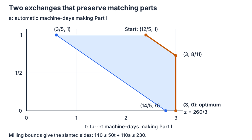
Use Next worked exchange twice at the published baseline to reproduce $78$, $900/11$, and $260/3$ (the lab rounds displayed decimals). Restore published baseline and replay resets both the capacities and the path. Changing capacities is a hypothetical experiment: the displayed optimum is recalculated, while the worked two-pivot replay is reserved for the original data. Zero capacity and invalid inputs have explicit status messages. Buttons and fields support keyboard use. The dictionaries and figure above remain usable without JavaScript.
Replay simplex exchanges on the published machine data
Published illustrative-data baseline: 3 milling, 3 turret, and 1 automatic machine-day, with the fixed Part I/II rates from Kantorovich, Example 1 and Table 1, p. 369. The allocations and exchanges are modern re-derivations using divisible time, full utilization, exact matching of parts, and no setup time. Fractional outputs are daily production rates. Capacity changes are hypothetical experiments.
The automatic lathe has the largest raw rate for both parts, yet the optimum assigns it only Part II. Reduced costs compare alternative uses after enforcing balance; raw productivity alone cannot do that.
Generalize the dictionary to any standard-form LP
Write the maximization problem in equality standard form, with $A\in\mathbb R^{r\times n}$ having independent rows:
\[\text{maximize }c^Tx\quad\text{subject to }Ax=b,\quad x\ge0.\]Here $r$ counts equations, $n$ counts variables, $A_j$ is column $j$, and $c_j$ is its objective coefficient. Split the variables into basic indices $B$ and nonbasic indices $N$. Let $M=A_B$ denote the invertible basis matrix. Then
\[x_B=\bar b-M^{-1}A_Nx_N,\qquad \bar b=M^{-1}b,\] \[c^Tx=z_0+\sum_{j\in N}\bar c_jx_j,\qquad z_0=c_B^T\bar b,\qquad \bar c_j=c_j-c_B^TM^{-1}A_j.\]These formulas follow by solving the constraint equations and substituting into the objective, exactly as in the machine dictionaries. See Goemans, §3. A minimization convention reverses the improving reduced-cost sign.
Assume $\bar b\ge0$, so the current basis is feasible. Choose $j\in N$ with $\bar c_j>0$. Set $x_j=\theta$ and all other nonbasic variables to zero. With $d=M^{-1}A_j$,
\[x_B(\theta)=\bar b-\theta d,\qquad z(\theta)=z_0+\theta\bar c_j.\]Only $d_i>0$ decreases a basic variable, so
\[\theta^{\star}=\min_{i:d_i>0}\frac{\bar b_i}{d_i}.\]A minimizing row identifies the leaving basic variable. The entering variable replaces its column; the nonzero pivot coefficient makes the replacement basis invertible. Recompute the dictionary and repeat. If every nonbasic reduced cost is nonpositive, the objective identity proves optimality. If $d_i\le0$ for all rows, the feasible ray $\theta\ge0$ improves without limit, proving unboundedness. These conclusions require a feasible starting basis; an infeasible tableau is not enough.
For a supplementary invented unbounded example, maximize $x_1$ subject to $x_1-x_2=1$ and $x_1,x_2\ge0$. The dictionary $x_1=1+x_2$, $z=1+x_2$ has no decreasing basic variable. Every point $(1+\theta,\theta)$ is feasible, with objective tending to infinity.
The same basis supplies a dual certificate
Define $y$ by $M^Ty=c_B$. At a basis with all $\bar c_j\le0$, the reduced-cost formulas imply $A^Ty\ge c$, with equality on basic columns. Because these are equality constraints, $y$ is unrestricted in sign. For any feasible $x$,
\[c^Tx\le y^TAx=y^Tb=c_B^TM^{-1}b=z_0.\]The current solution attains this bound. This is the basis connection to duality; see MIT’s “Simplex and Duality” discussion.
For the historical model, order the four rows as part balance, milling capacity, turret capacity, automatic capacity. The final basis gives
\[y=\left(\frac13,0,\frac{10}{3},0\right),\qquad b=(230,3,3,1)^T,\qquad b^Ty=\frac{260}{3}.\]The nonbasic columns $a$ and $s_t$ have $A_j^Ty-c_j=20/3$ and $10/3$, respectively. These are the negatives of their final reduced costs. The zero automatic-capacity multiplier does not mean extra automatic machinery is worthless: additional automatic time also changes the part-balance constant $230$. A physical capacity change must update both right-hand sides, as the final exercise shows.
Phase I: find a feasible basis before optimizing output
The historical starting corner was easy to find. An arbitrary LP may have no obvious feasible basis. First make right-hand sides nonnegative by multiplying any row with $b_i<0$ by $-1$. Add nonnegative artificial variables $u_i$, one per equation, to obtain
\[Ax+u=b,\qquad x,u\ge0,\qquad \text{minimize }w=\sum_{i=1}^{r}u_i.\]The artificial columns form an identity matrix, so $x=0,u=b$ is a feasible basis for this auxiliary problem. Artificial variables measure equation discrepancies in this construction; they are not physical production activities. Phase I solves this problem (equivalently maximize $-w$). Its optimum is nonnegative. If it is positive, the original equations have no nonnegative solution; if it is zero, $u=0$ gives an original feasible point. Pivot zero artificial basic variables out, removing redundant zero rows if necessary, then restore and re-express the original objective for Phase II. See Goemans, §2.5.
For a supplementary invented infeasible system, require $x\ge2$ and $x\le1$. With surplus $s_1\ge0$ and slack $s_2\ge0$, use
\[x-s_1+u_1=2,\qquad x+s_2+u_2=1,\qquad w=u_1+u_2.\]The second equation forces $x\le1$. The first gives $u_1=2-x+s_1\ge1$. Thus $w\ge1$, attained at $(x,s_1,s_2,u_1,u_2)=(1,0,0,1,0)$. The positive Phase I optimum proves infeasibility. Farkas’ lemma explains how a contradiction certificate can express the same conclusion.
Degeneracy changes what a pivot means
A BFS is degenerate when at least one basic variable is zero. In that case the ratio test may return $\theta^{\star}=0$: a positive reduced cost need not give a strict improvement. Distinct bases can represent the same point.
For a supplementary invented example, maximize $x_1+x_2$ subject to $x_1\le1$, $x_2\le1$, $x_1+x_2\le1$, and nonnegativity. At $(1,0)$, choose basic variables $(x_1,s_2,s_3)$ and nonbasic $(x_2,s_1)$. The dictionary includes
\[x_1=1-s_1,\qquad s_2=1-x_2,\qquad s_3=s_1-x_2,\qquad z=1-s_1+x_2.\]Although $x_2$ has reduced cost $1$, with $s_1=0$ the row $s_3=-x_2$ permits only a zero step. Pivoting $x_2$ in and $s_3$ out changes the basis but leaves $(x_1,x_2)=(1,0)$. This point was already optimal because $x_1+x_2\le1$. Thus nonpositive reduced costs suffice for optimality, but a degenerate basis at an optimal point need not initially have that sign pattern.
Repeated zero steps can cycle under unsuitable rules. Bland’s rule fixes an ordering of all variables, selects the smallest-index eligible entering variable, and among minimum-ratio ties selects the smallest-index basic variable to leave. In exact arithmetic this prevents cycling and gives finite termination. See Goemans, §2.4.2, Theorem 2.2. Finite does not mean few: particular simplex rules have exponential worst cases. See MIT’s discussion of Klee–Minty examples.
The geometric simplex (nonnegative coordinates summing to one) is a particular feasible set; the simplex algorithm applies far beyond that set. The machine polygon need not be a triangle. Also, simplex solves a continuous LP: fractional optimal machine-days do not automatically solve an integer scheduling problem.
Implement the algebra with linear solves
The inverse notation explains the derivation, but a revised simplex implementation works with the basis matrix and solves systems for basic values, prices, and directions. See Goemans, §3. In particular, compute $M\bar b=b$, $M^Ty=c_B$, and $Md=A_j$ using a factorization such as LU decomposition. Reusing factors avoids explicitly forming the inverse.
The practical checks follow directly from the equations: verify $Ax-b$, nonnegativity, the reduced-cost signs, and the primal–dual objective gap. Floating-point tolerances must account for the scale of the rows and columns; near-zero pivots and nearly tied ratios need care. A tiny residual alone does not establish a small solution error. The worked derivations here use exact fractions; the interactive lab uses floating-point arithmetic and rounded displays.
Practice problems
These original exercises include hand calculation, interpretation, logical reasoning, and a practical capacity calculation. The first, second, and fourth use the published machine rates in our continuous model.
1. Hand calculation: recover the first pivot
From the initial dictionary, choose $s_a$ to enter. Identify every decreasing basic variable, compute the ratios, and find the new point and objective gain.
Hint
Hold $m=0$. A positive coefficient in a basic row means that basic variable increases, so it does not limit the step.
Worked solution
$s_t$ decreases at rate $11/5$ and $a$ at rate $1$. Their ratios are $(3/5)/(11/5)=3/11$ and $1$. The variables $t$ and $s_m$ increase or stay fixed. Thus $s_t$ leaves at $s_a=3/11$. The new point is $(m,t,a)=(0,3,8/11)$, and $z=78+14(3/11)=900/11$. The gain is $42/11$ complete sets per day.
2. Interpretation: a larger reduced cost versus a longer move
At the initial dictionary, a planner proposes increasing $s_a$ to $1$ because its reduced cost is positive. Which constraint fails? Why does the reduced cost not authorize that choice?
Hint
Substitute $s_a=1,m=0$ into both the turret row and its slack row.
Worked solution
The proposed values give $t=23/5>3$ and $s_t=-8/5<0$. The reduced cost $14$ is an objective slope along an equality-preserving direction; it does not remove the nonnegativity constraints. Only $0\le s_a\le3/11$ is feasible with $m=0$. Step length and objective slope must both be considered.
3. Logical reasoning: can a zero reduced cost prove multiple optima?
At an optimal dictionary, suppose a nonbasic variable has zero reduced cost. Does that alone prove another distinct optimal point exists? State an additional sufficient condition and give a counterexample without it.
Hint
The objective stays fixed along this direction. Ask whether a positive step is possible.
Worked solution
No. A positive feasible step along that direction suffices: it changes the entering coordinate while preserving the optimal value. A supplementary counterexample is $\max 0$ subject to $x+s=0$, $x,s\ge0$. With $s$ basic, the dictionary is $s=-x$, $z=0$. The nonbasic reduced cost is zero, but the sole feasible point is $(0,0)$; its maximum step is zero. A zero-step pivot alone does not establish distinct optimal solutions.
4. Application: how long does the old capacity price remain valid?
Add $\delta\ge0$ automatic machine-days while keeping the published production rates and the other capacities fixed. Continue the specialization $t=3,a=0$. Find $m$, the output, and the range of $\delta$ for which this plan still reaches the bound supplied by the old multipliers.
Hint
The balance constant becomes $230+80\delta$ and automatic capacity becomes $1+\delta$. Both entries of $b$ change.
Worked solution
Balance gives $30m+150=230+80\delta$, hence $m=8/3+(8/3)\delta$. Output is $z=10m+60=260/3+(80/3)\delta$. Feasibility requires $m\le3$, so $0\le\delta\le1/8$. The old dual vector stays feasible because $A,c$ are unchanged, and its bound changes by $(1/3)(80\delta)+0\delta=(80/3)\delta$. The plan attains that bound throughout this range. Beyond it, the formula violates milling capacity and cannot predict the optimum. The endpoint makes $s_m=0$, producing a degenerate basis where the specialization can change.
References and further learning
- L. V. Kantorovich, Mathematical Methods of Organizing and Planning Production (1939; English translation, 1960): Example 1 and Table 1, pp. 369–370, supply the published illustrative rates; Problem A states the full-use matching model. The simplex dictionaries here are modern derivations using those data.
- Michel X. Goemans, MIT 18.310, Linear Programming notes (2015): §§2.3–2.5 develop pivots, degeneracy, Bland’s rule, and Phase I; §3 gives the matrix formulation. Useful for connecting dictionaries to tableaus and implementing the basis equations.
- MIT 6.854, Lecture 14, Algorithms for Solving LPs (2020): connect basis geometry, reduced costs, dual certificates, and worst-case limitations.
- Linear programming: study model construction, the historical assignment problem, and alternative LP methods.
- Duality and Farkas’ lemma: understand optimality bounds and proofs of infeasibility.